#' The Probability Density for the Correlation Coefficient for
#' Uncorrelated Normal Distributions
#'
#' @param r The observed Pearson correlation
#' @param n The sample size
#'
#' @details
#' More details can be found here:
#' <https://en.wikipedia.org/wiki/Pearson_correlation_coefficient#Using_the_exact_distribution>
#'
#' A more complicated formula exists for the density of Pearson
#' correlation statistics calculated from bivariate normal
#' distributions with rho != 0.
#'
#' The reason for the inclusion of a normalizing constant was that I found that
#' integrating from -1 to 1 for positive integers n was not reflecting properly that
#' P(r in [-1,1]) = 1.
#'
cor_coef_density <- function(r, n) {
unnormalized_density <- function(r, n) {
(1/(1-r^2))^{-(n-1)/2} / (sqrt(n-2) * beta(1/2, (n-2)/2))
}
normalizing_constant_for_n <- integrate(f = unnormalized_density, lower = -1, upper = 1, n = n)[[1]]
return(unnormalized_density(r, n) / normalizing_constant_for_n)
}
# Probability of observing correlation coefficient of at least .25:
integrate(f = cor_coef_density, lower = 0.25, upper = 1, n = 100)
integrate(f = cor_coef_density, lower = 0.25, upper = 1, n = 20)
# In either sample sizes of 100 or 25, the probability of observing a
# Had to correct for the normalizing constant...
integrate(f = cor_coef_density, lower = -1, upper = 1, n = 20)
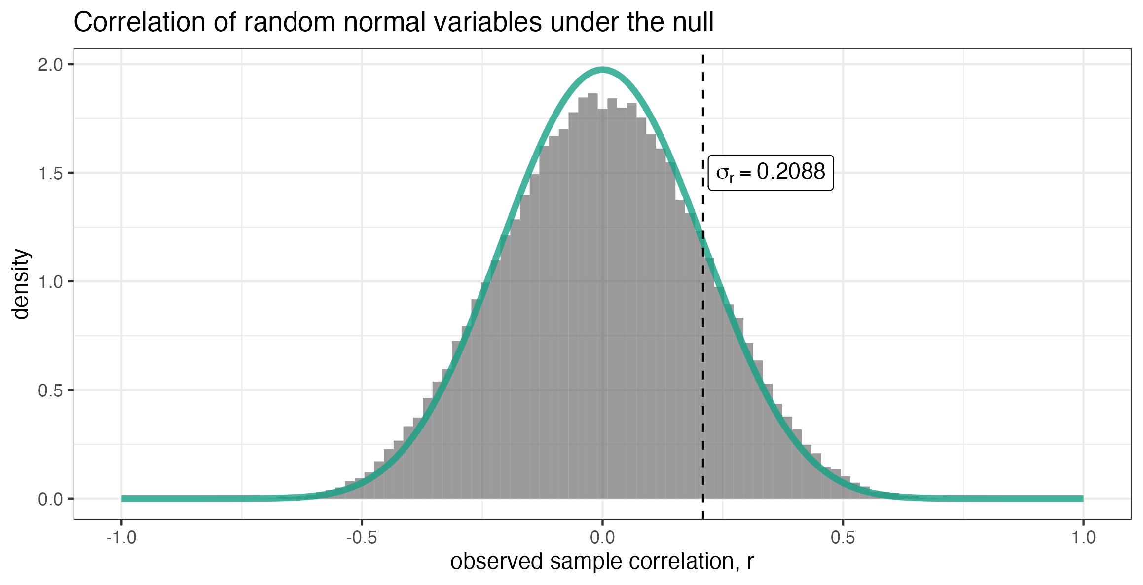
# Now check if it's right under a simulation study
n <- 24L
n_sims <- 100000L
observed_r <- numeric(length = n_sims)
for (i in 1:n_sims) {
X <- rnorm(n = n)
Y <- rnorm(n = n)
observed_r[i] <- cor(X,Y)
}
sd(observed_r)
library(ggplot2)
# looks like perhaps the approximation is slightly off? but it looks largely
# correct — and importantly, it seems to covary with the population size in the
# right way
ggplot() +
geom_histogram(
data = data.frame(observed_r = observed_r),
mapping = aes(x = observed_r, y = ..density..),
bins = 100, alpha = 0.6) +
geom_line(
tibble::tibble(
x = seq(-1,1,length.out=1000),
y = cor_coef_density(r = x, n = n)),
mapping = aes(x = x, y = y),
linetype = 'solid', color = '#16a085', linewidth=1.5, alpha = 0.8) +
geom_vline(
xintercept = 0.2088,
linetype = 'dashed') +
annotate(
geom = 'label',
label = expression(sigma[r] == "0.2088"),
x = .35,
y = 1.5) +
labs(x = "observed sample correlation, r", y = 'density') +
ggtitle("Correlation of random normal variables under the null") +
theme_bw() Who was Charles Spearman?
- Known for his work in psychology, Spearman was born in London in 1863 and died in 1945. His most famous work was on human intelligence
- He served in the army from 1883 to 1897, and then went to study at the University of Leipzig, where he was influenced by Wilhelm Wundt, the father of experimental psychology, or “new psychology”
- I.e., used empirical methods instead of metaphysical reasoning
- He was recalled to the army during the Second Boer War and served as a general
- Somehow, amidst all this, he published his most famous work in 1904

Who was Charles Spearman?
- Spearman was heavily persuaded by Galton’s work, particularly the creation of “Co-relation” from 1888.
- See, for example, Stigler’s 1989 article Francis Galton’s Account of the Invention of Correlation
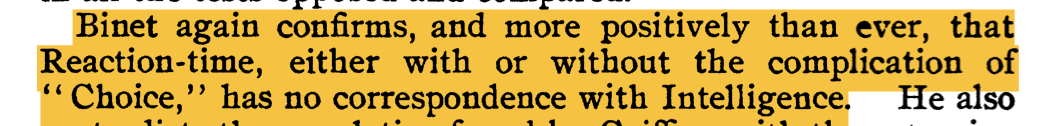
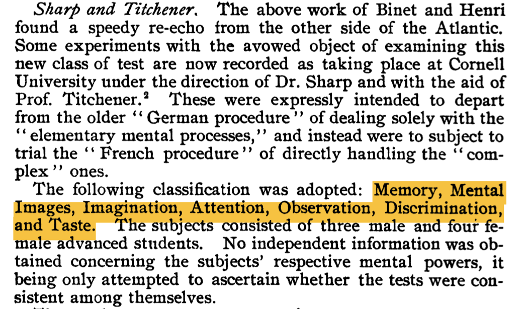
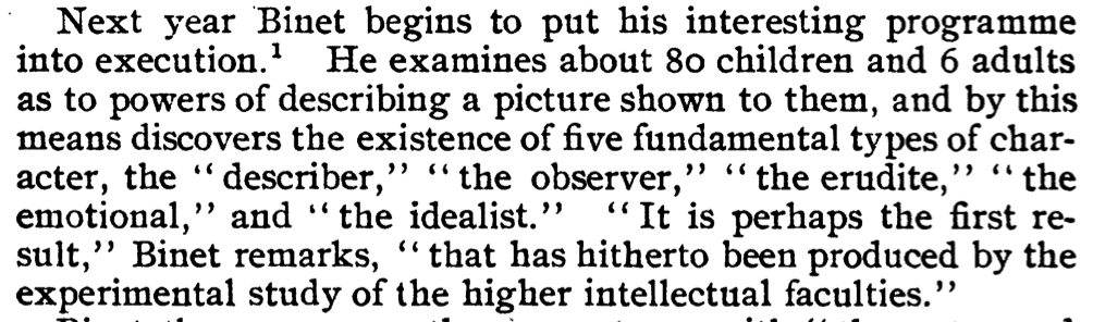
- He was also influenced by the work of the French psychologist Alfred Binet, who was working on the first intelligence tests, e.g., “intelligence quotients”
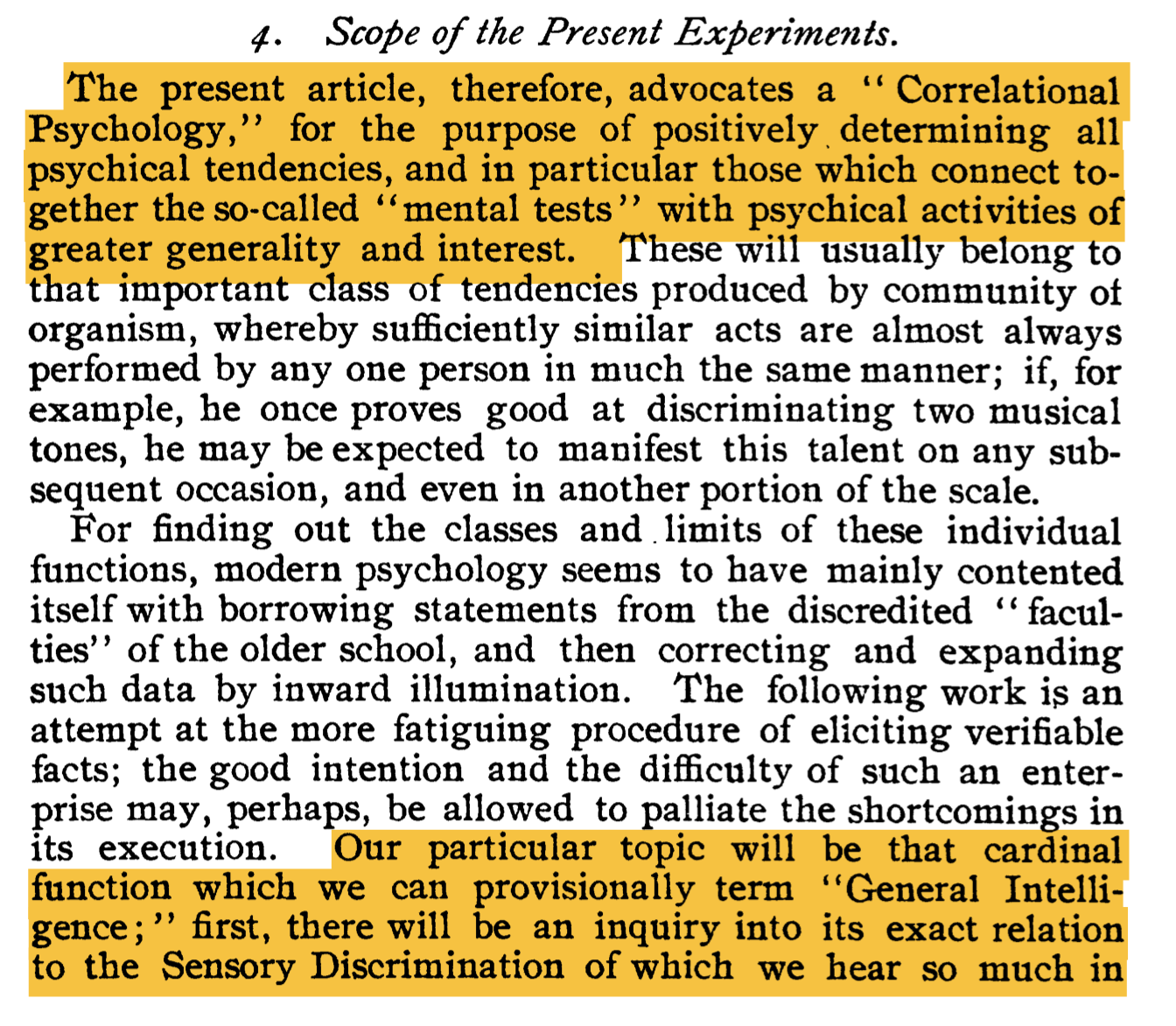
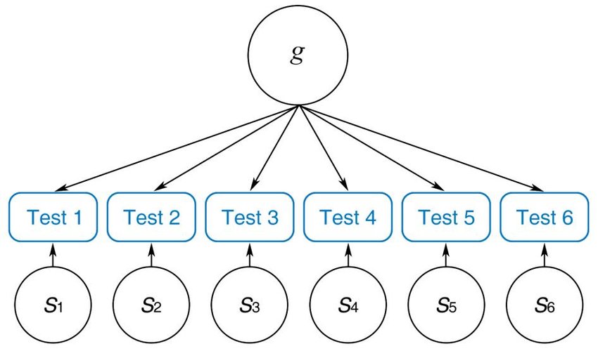
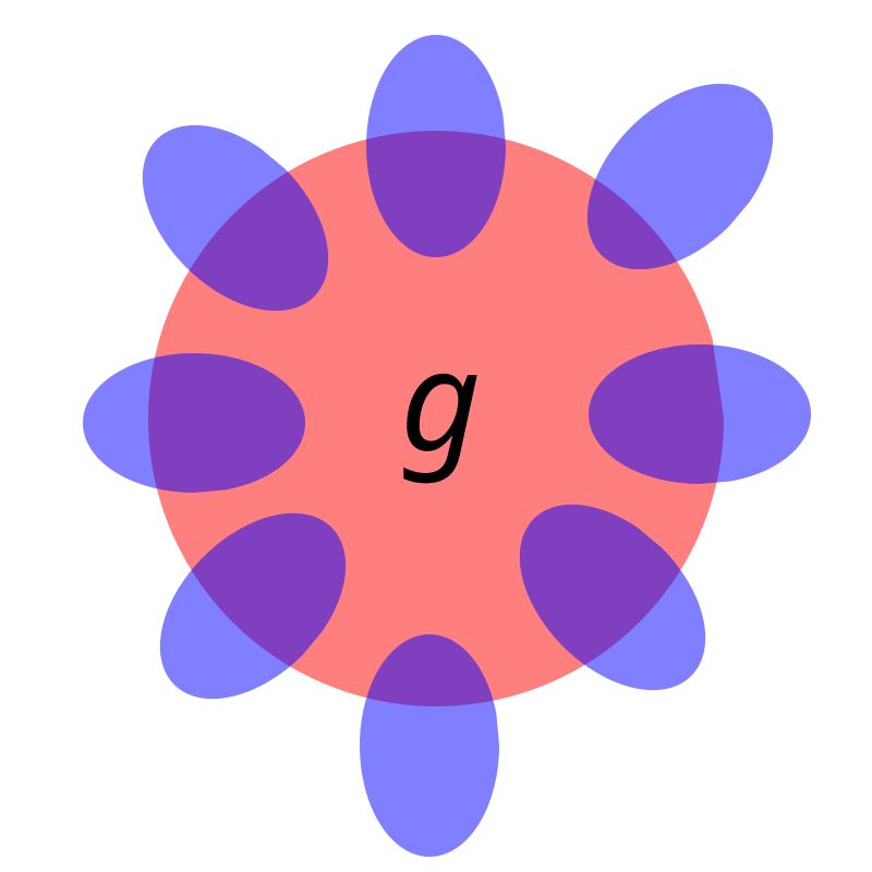
- His seminal 1904 work posits that intelligence rests on a single, general (latent) factor, which he called “g”
- This was the first work in the field now called factor analysis
- He also developed rank correlation
What were his motivations in writing?
He sees psychology as an up-and-coming field, and yet also a subject looked down-upon by the scientific community.
He’s trying to make a case for psychology as a science, rooted in data analysis and empirical methods.
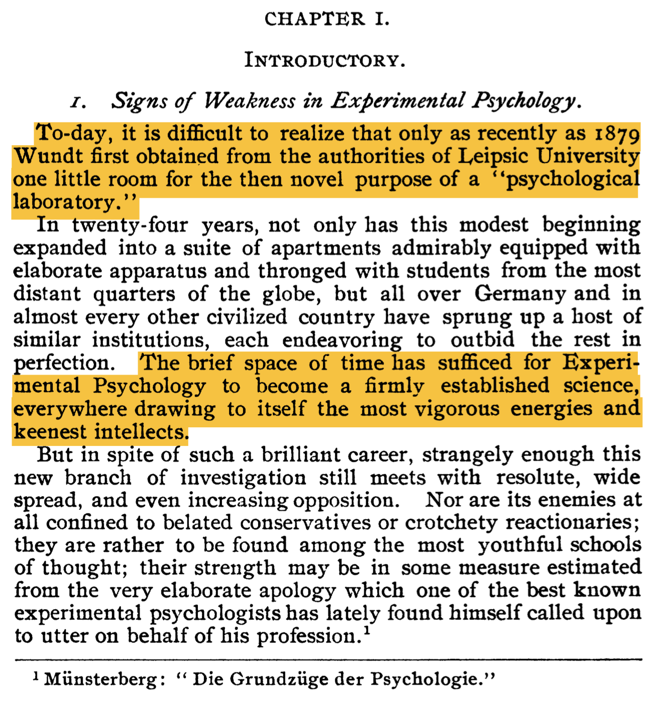
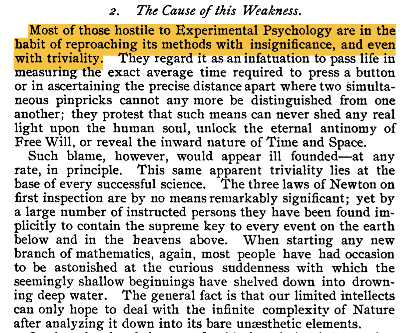
What were his motivations in writing?
He is making clear he intends to lay down the scientific foundations of psychology, which will be (implicitly) comparable to Newton’s equations of motion —
Especially with an eye towards refuting the criticisms of psychology as puttering about.
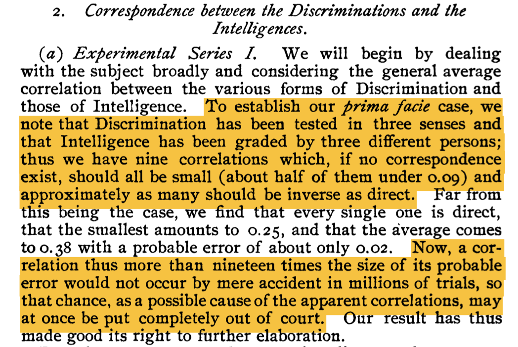
What were his main arguments?
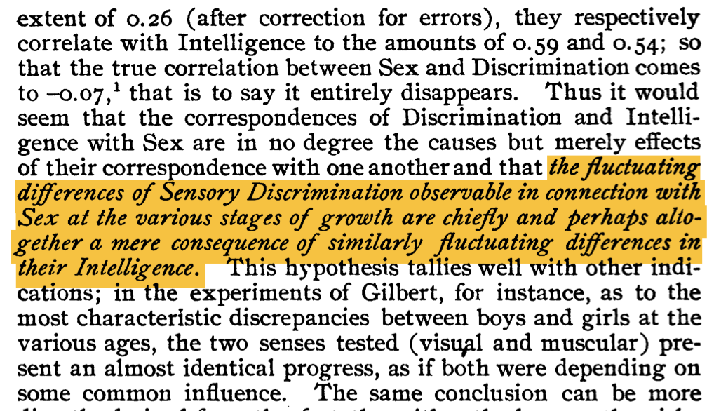
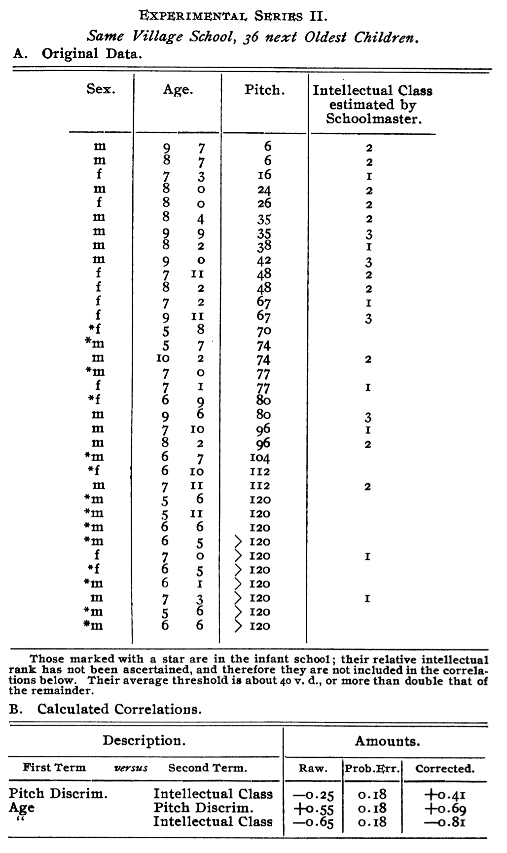
Spearman was analyzing data on children’s performance across various school tests, and he found that the scores were correlated.
In analyzing the data and their correlations, he hypothesized that there was a single, general factor that was responsible for the correlations and he called this the “g” factor.
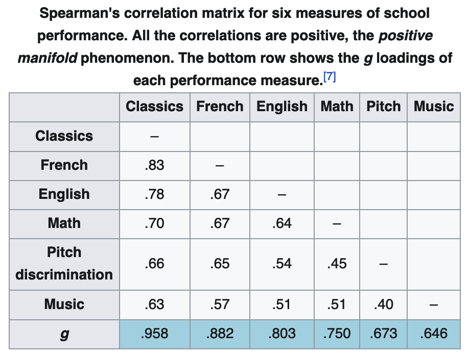
What were his main arguments?

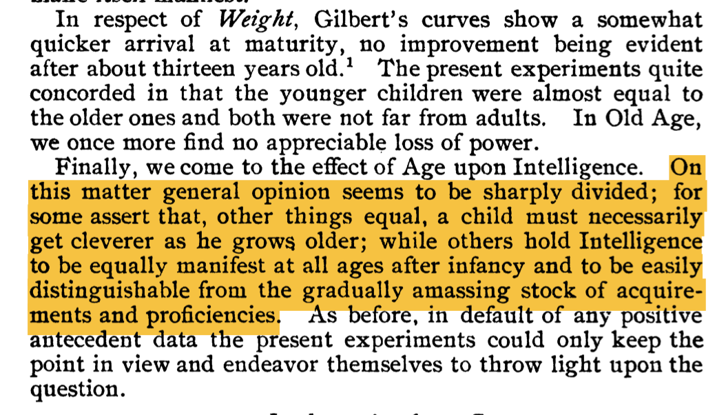
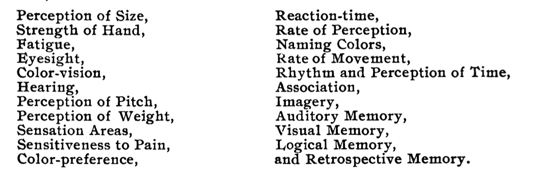
State of the art in 1904
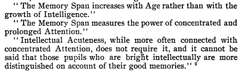
State of the art in 1904
State of the art in 1904
State of the art in 1904
State of the art in 1904
State of the art in 1904
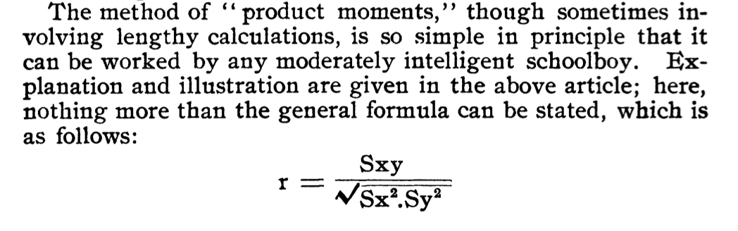
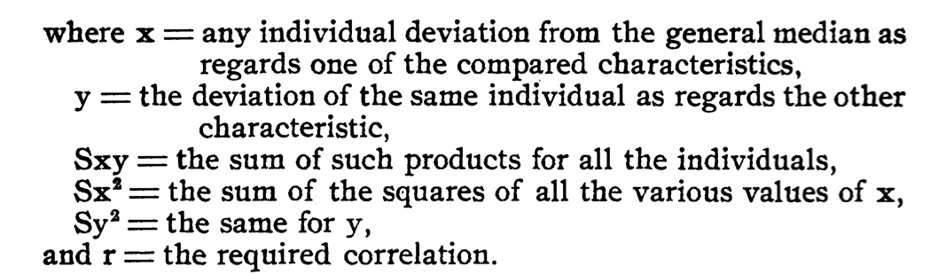
Correlation
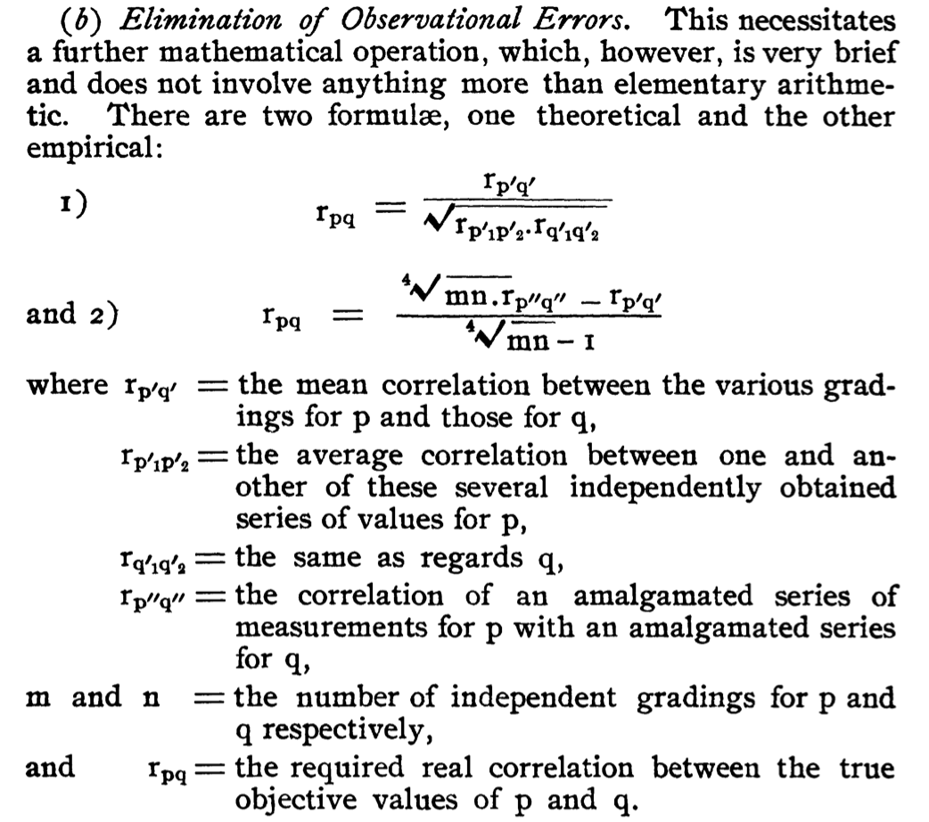
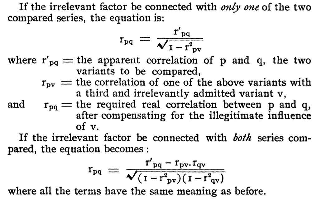
Correlation — Elimination of Observational Errors
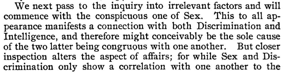
Correlation — Elimination of Irrelevant Factors
Experiment I
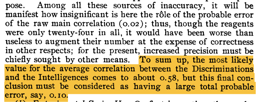
Checking his math
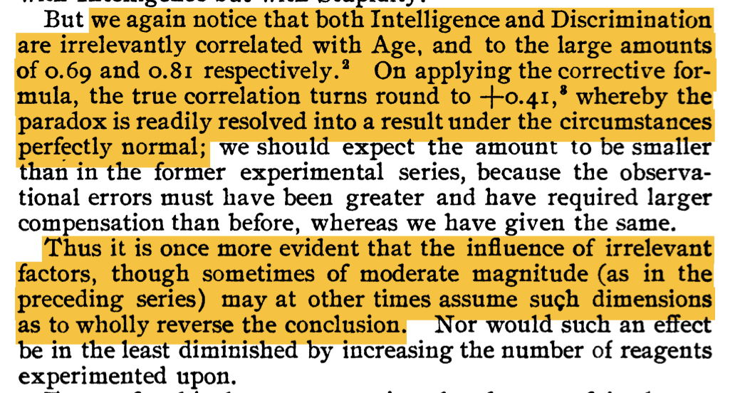
Adjusting for “irrelevant factors”
Conclusions from Experiment I
Experiment II
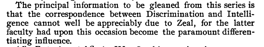
Experiment III
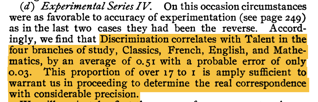
Experiment IV
Conclusions of Experiments
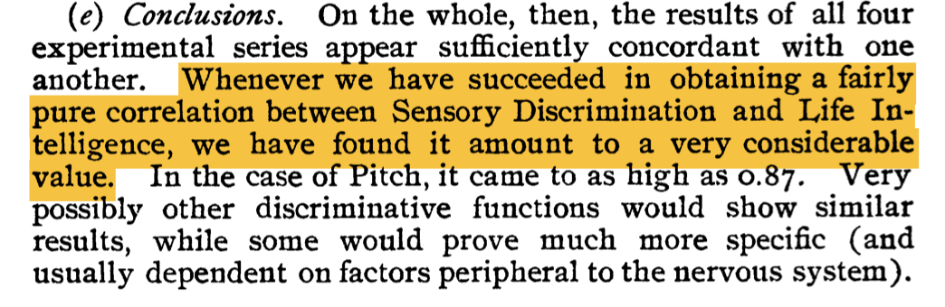
Interpretation
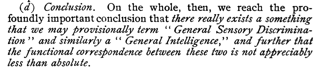
Conclusions of Experiments
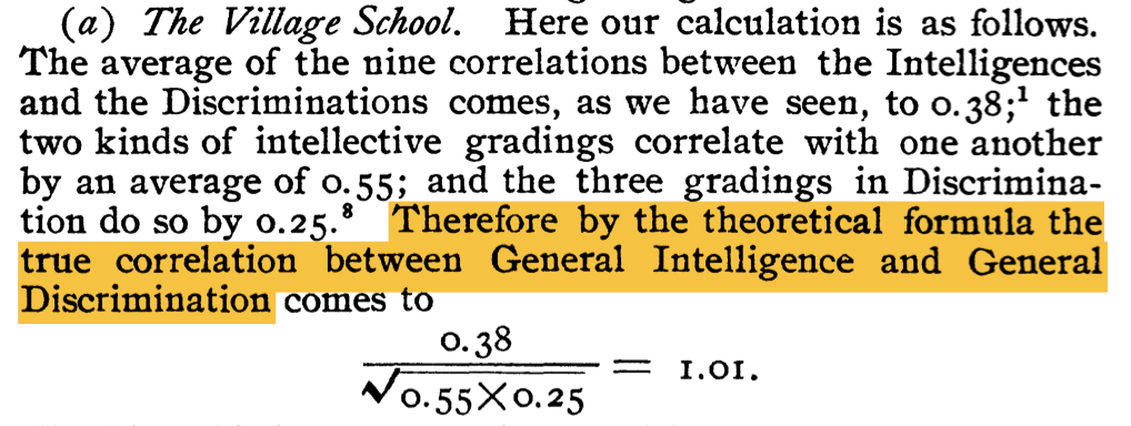
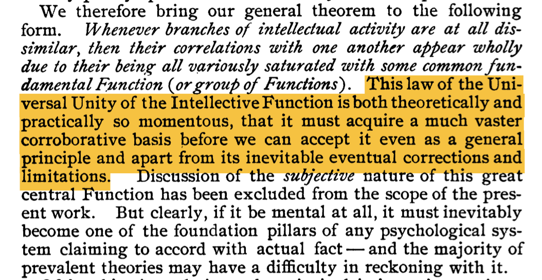
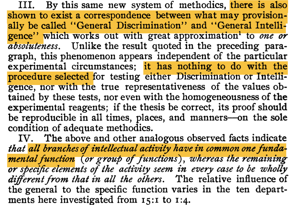
A “Theorem”
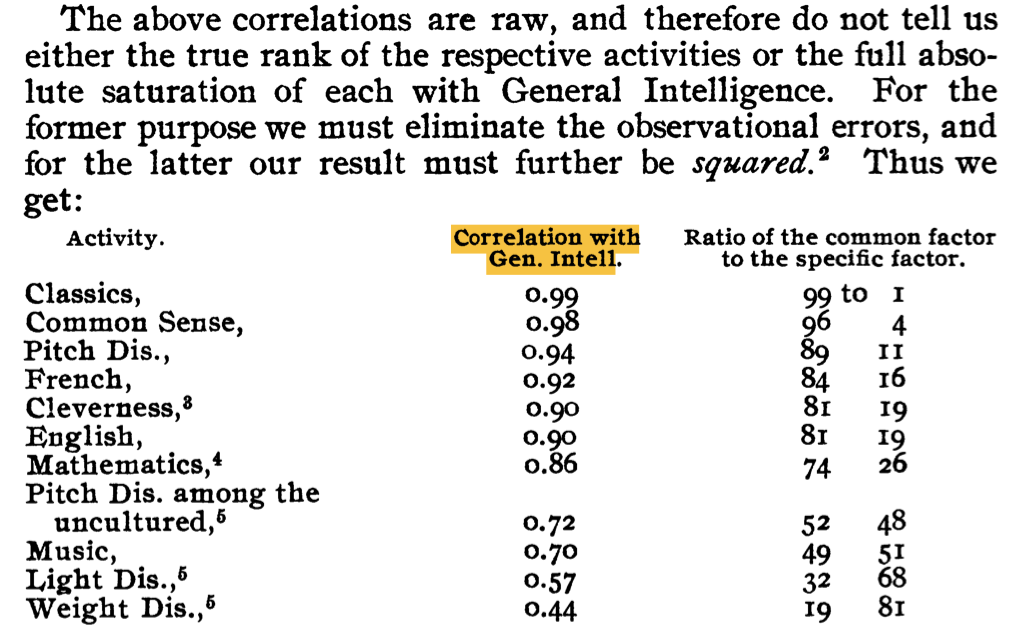
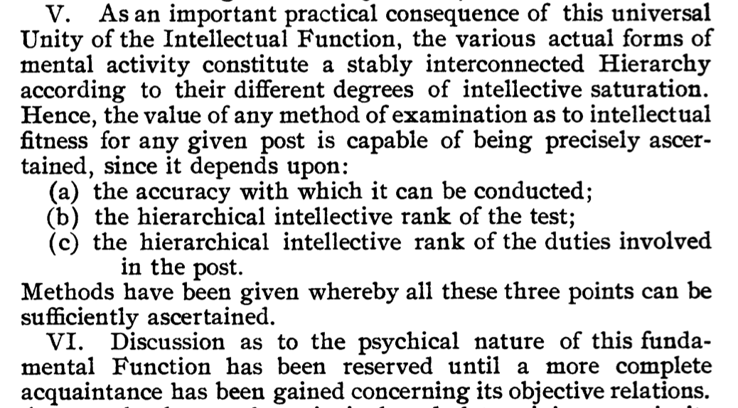
Hierarchy of Factors
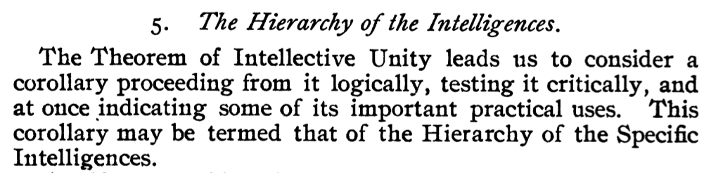
Hierarchy of Factors
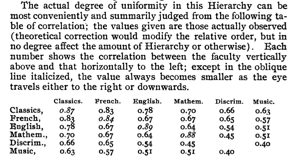
Hierarchy of Factors
His Discussion
His Discussion
Appendix
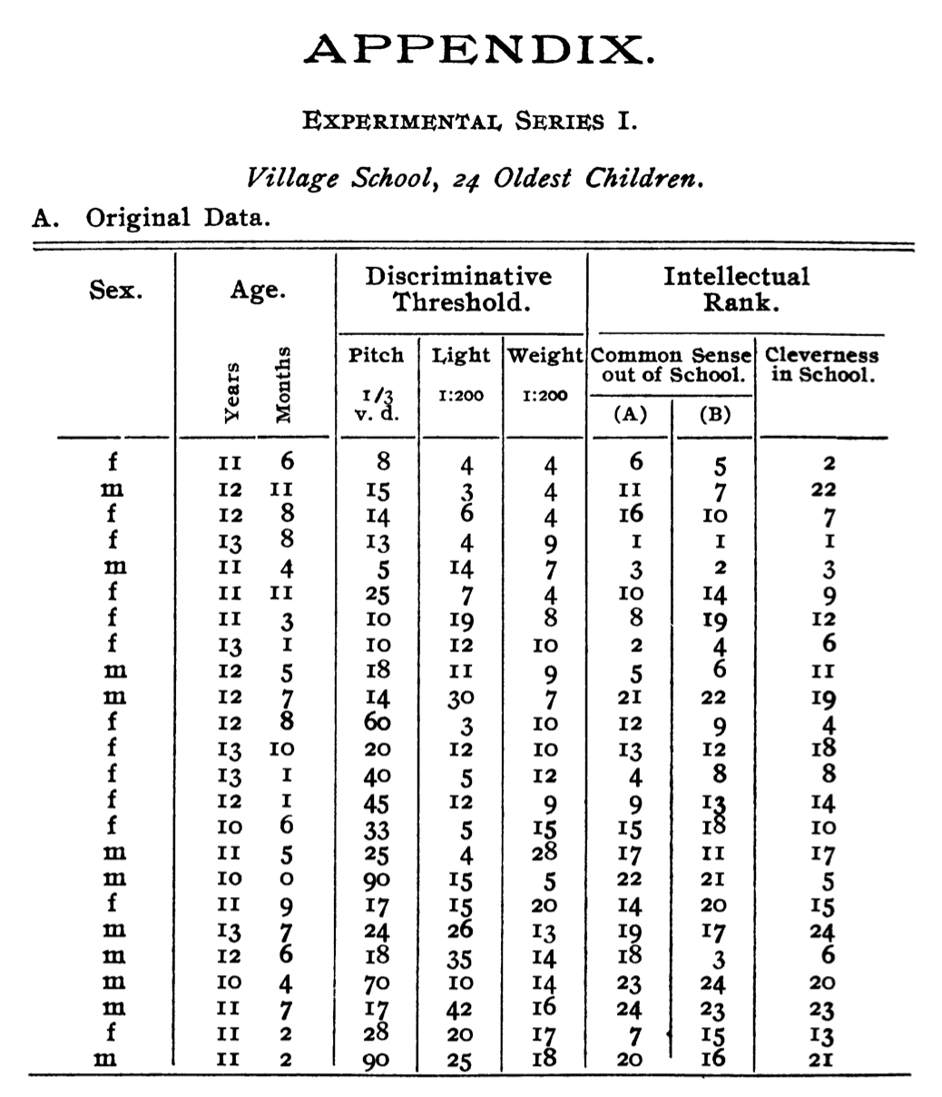
Appendix
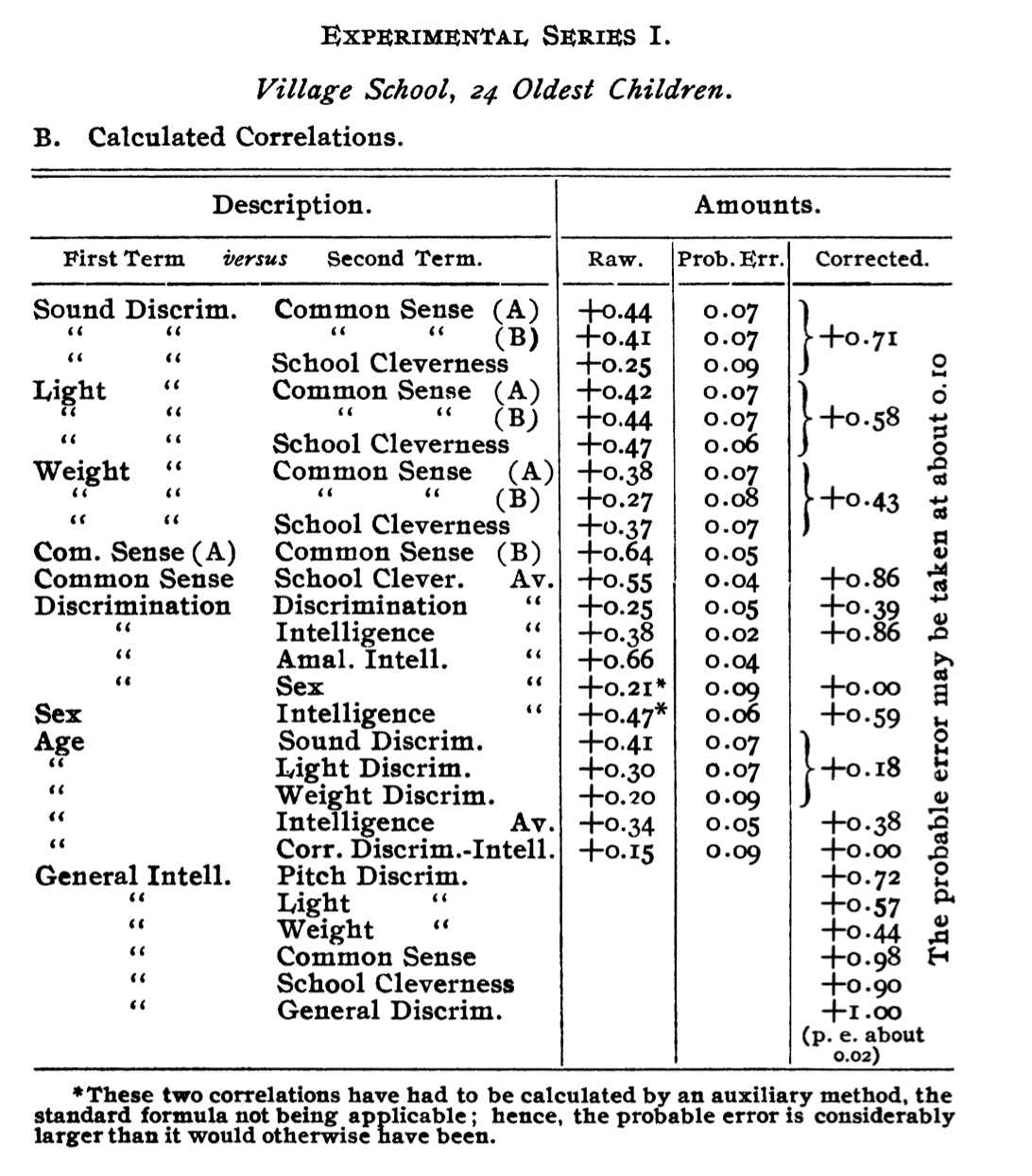
Appendix
Contemporary Uses of Factor Analysis
Factor analysis has since been used in many fields, but especially psychology. It is common to see factor analysis in survey analysis (Qualtrics has a guide).
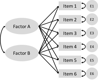
One workflow is to have respondents rate their agreement with a series of statements, then latent factors are identified from the responses using factor analysis, and factor scores describe how much variance of each observed variable is explained by each of the latent factors.
Spearman’s work only posited the existence of one common factor for intelligence measures, but after its development by Thurstone in the 1930-50s, factor analysis with multiple factors is now common.
Example
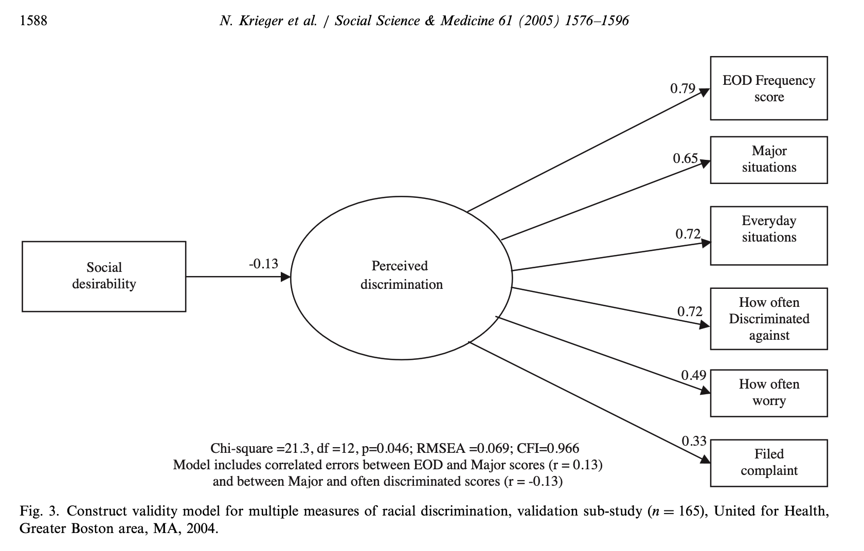
Krieger, N., Smith, K., Naishadham, D., Hartman, C., & Barbeau, E. M. (2005). Experiences of discrimination: validity and reliability of a self-report measure for population health research on racism and health. Social science & medicine (1982), 61(7), 1576–1596. https://doi.org/10.1016/j.socscimed.2005.03.006
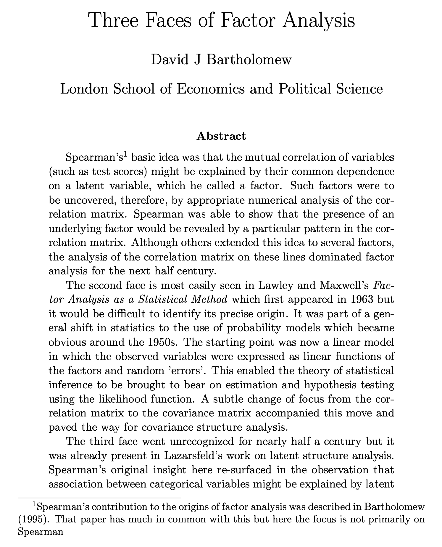
Bartholomew, 2007
Bartholomew, D. J. (2007). Three faces of factor analysis. In R. Cudeck & R. C. MacCallum (Eds.), Factor analysis at 100: Historical developments and future directions (pp. 9–21). Lawrence Erlbaum Associates Publishers.
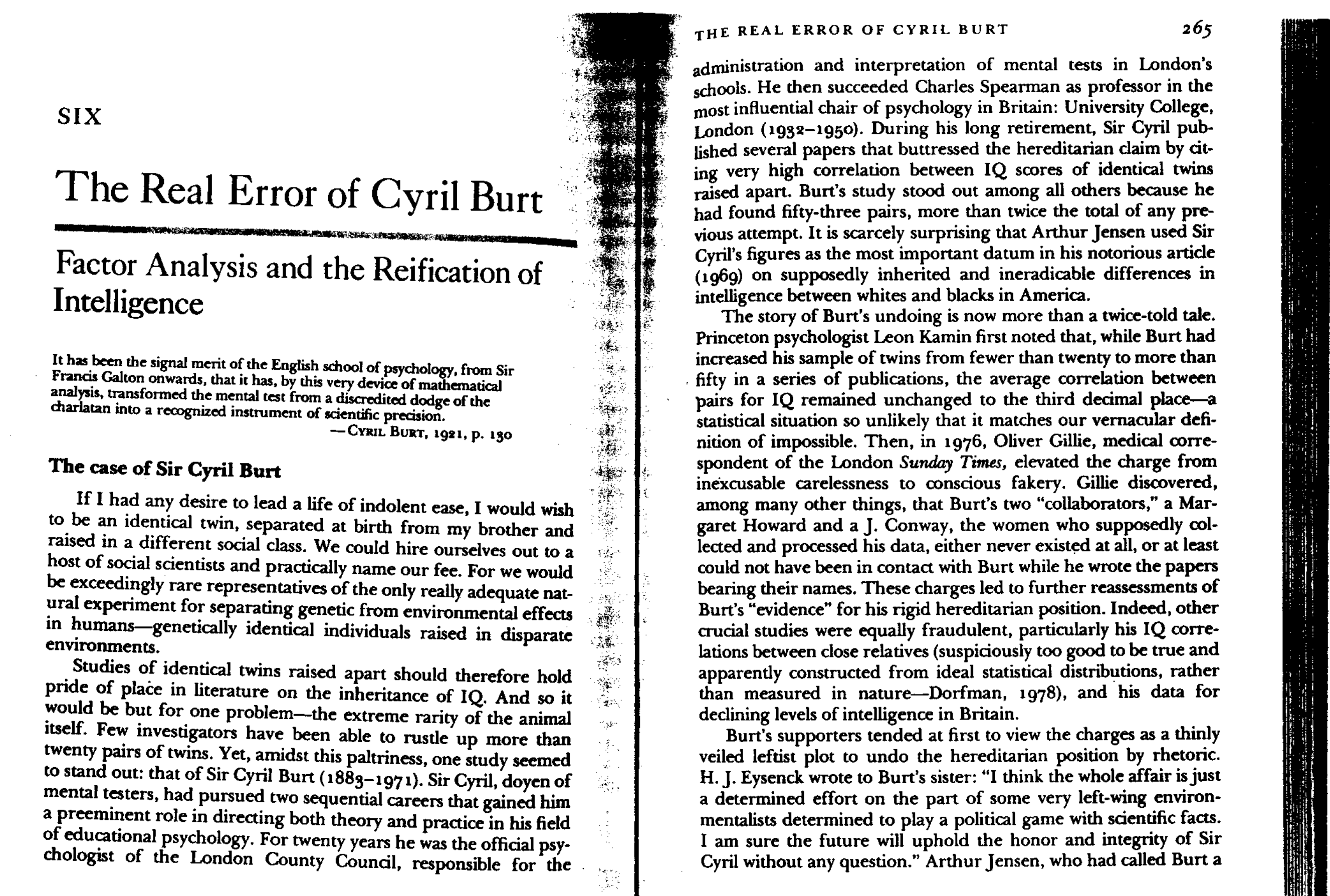
Gould, 1981
Gould, S. J. (1981). Mismeasure of Man. New York: Norton & Company
Chapter 6: The Real Error of Cyril Burt
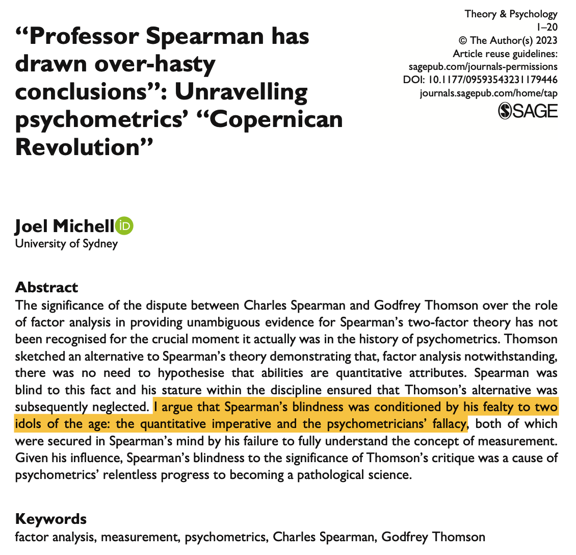
Michell, 1997
Michell, J. (2023). “Professor Spearman has drawn over-hasty conclusions”: Unravelling psychometrics’ “Copernican Revolution”. Theory & Psychology, 33(5), 661–680. https://doi.org/10.1177/09593543231179446
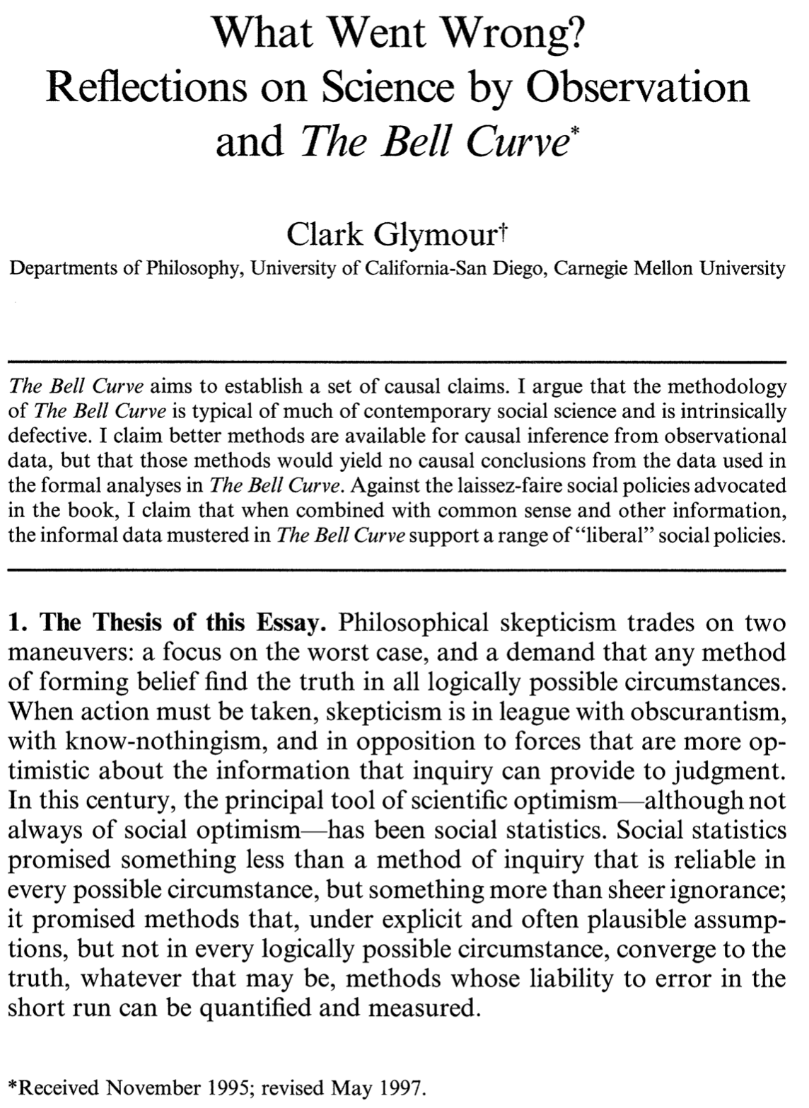
Glymour, 1998
Glymour, Clark. “What Went Wrong? Reflections on Science by Observation and the Bell Curve.” Philosophy of Science, vol. 65, no. 1, 1998, pp. 1–32. JSTOR, http://www.jstor.org/stable/188173.