Comparing Estimators
Comparing-Estimators.RmdA famous example of a statistical inference problem where a faster than rate of convergence is possible is that of inferring the parameter in a model.
We will show how a moments based estimator converges slower than an order statistic based estimator empirically using Simulacron3.
For our first estimator, we will take
Our second estimator will be
library(Simulacron3)
suppressMessages(library(dplyr))
library(ggplot2)
library(tidyr)

# we can fix a true value or even set it to be random as long as we record it.
theta <- 10

# here's our data generating process (dgp):
unif_dgp <- function(n) {
  runif(n = n, min = 0, max = theta)
}

# here are our two candidate estimators that we want to compare across simulations
estimator1 <- function(x) {
  sqrt(3/length(x) * sum(x^2))
}
estimator2 <- function(x) {
  (length(x)+1)/(length(x)) * max(x)
}

# our summary is just going to be to retrieve the estimators from each simulation
summary_func <- function(iter = NULL, est_results, data = NULL) {
  data.frame(
    estimator1 = est_results$estimator1,
    estimator2 = est_results$estimator2)
}

# setup our simulation
sim <- Simulation$new()
sim$set_dgp(unif_dgp)
sim$set_estimators(list(estimator1 = estimator1, estimator2 = estimator2))
sim$set_summary_stats(summary_func)

# setup a data frame to store results in across sample sizes
results <- list()

# run the simulation over a variety of sample sizes
sample_sizes <- c(10, 30, 100, 300)
results <- Simulacron3::run_simulation_study(sim, sample_sizes)

# combine our results together and pivot for ggplot2
results <- results |>
  tidyr::pivot_longer(
    cols = starts_with('estimator'),
    values_to = 'estimate',
    names_to = 'estimator'
  )

# produce a nice ggplot2 of the simulation results
results |>
  mutate(estimator_name = case_when(
    estimator == 'estimator1' ~ c(bquote(hat(theta)[1])),
    estimator == 'estimator2' ~ c(bquote(hat(theta)[2]))
  )) |>
  ggplot(aes(
    x = factor(sample_size),
    y = estimate,
    color = estimator,
    shape = estimator
  )) +
  geom_jitter(
    position = position_jitterdodge(dodge.width = .35,
                                    jitter.width = .10),
    alpha = .7) +
  geom_boxplot(outlier.color = NA,
               alpha = 0.5,
               width = .35) +
  theme_bw() +
  scale_color_brewer(
    palette = 'Set2',
    labels = c(estimator1 = bquote(paste(hat(theta)["n, moments"])),
               estimator2 = bquote(hat(theta)["n, max"]))) +
  scale_shape_discrete(
    labels = c(estimator1 = bquote(paste(hat(theta)["n, moments"])),
               estimator2 = bquote(hat(theta)["n, max"]))) +
  ggtitle("Comparison of Estimators",
          "100 simulations at each sample size were performed") +
  labs(x = "Sample Size", y = "Estimate")  +
  theme(legend.position = 'bottom')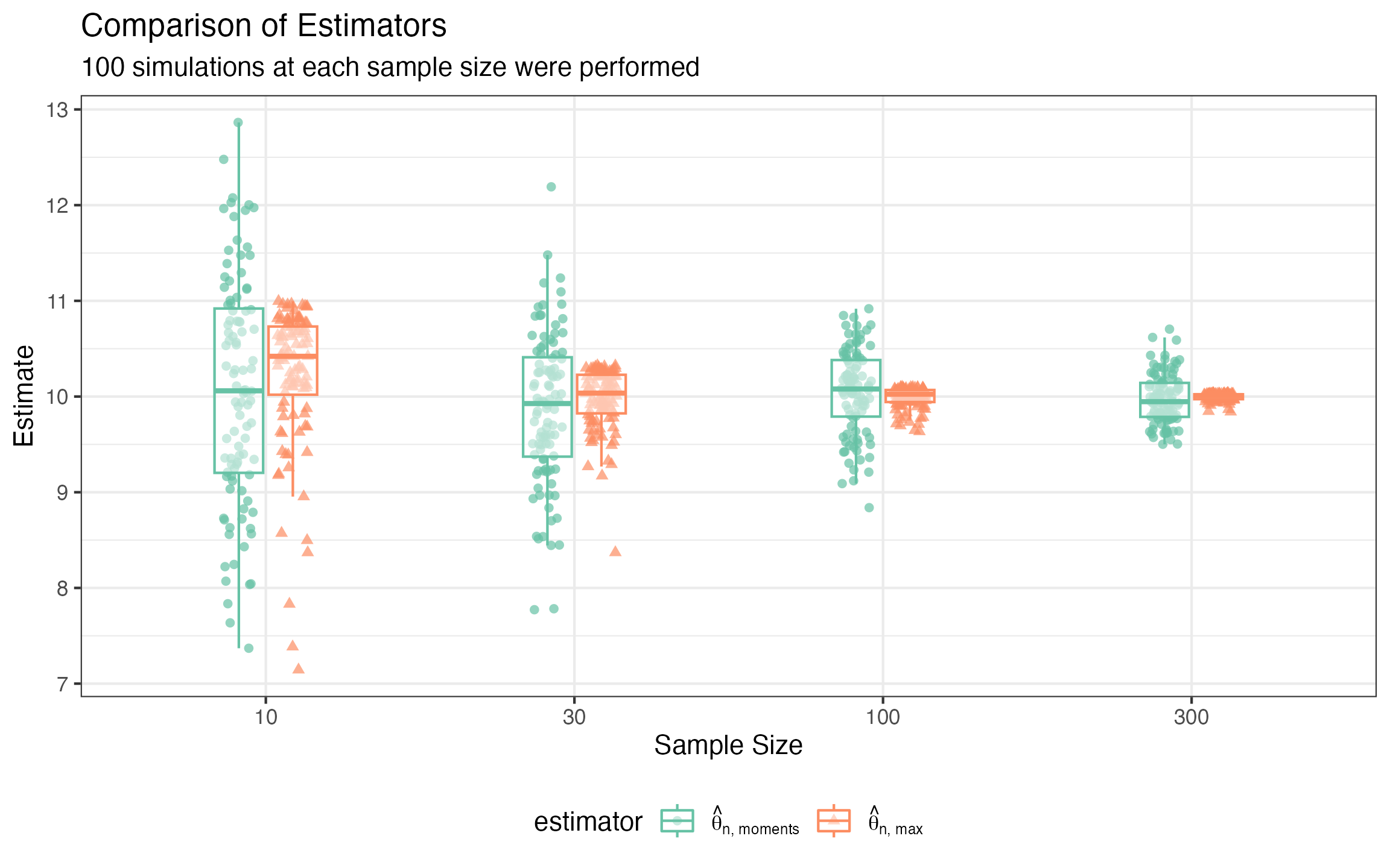
We can see that we were right to expect from theory that
estimator2 or
would converge quite a bit faster than estimator1 or
.