Benchmarking Against `{SuperLearner}` and `{sl3}`
Source:vignettes/articles/Benchmarking.Rmd
Benchmarking.RmdIt would be nice to compare SuperLearner
sl3 and nadir on some small, medium, and
large-ish datasets to see how they compare in timing results. For now,
we’ll start with some smaller ones to see how long it takes to get
super_learner() and cv_super_learner() (and
their equivalents) to run on these.
For these different sizes, I’d consider
-
irisas the small example (7.3 KB) -
penguinsfrom palmerpenguins as another small-ish example (16.8 KB) -
tornadosfrom tidytuesdayR 2023-05-16 (2.7 MB)
We’re running these on my laptop with 10 cores.
In all of these, we’ll use the same library of learners:
lnr_meanlnr_lmlnr_rflnr_earthlnr_glmnetlnr_xgboost
and their equivalents in the other packages.
iris data
library(pacman)
p_load('nadir', 'sl3', 'SuperLearner', 'microbenchmark', 'tidytuesdayR', 'future', 'ggplot2', 'forcats', 'dplyr')

# setup multicore use
future::plan(future::multicore)

petal_formula <- Petal.Width ~ Sepal.Length + Sepal.Width + Petal.Length + Species
nadir::super_learner() on iris (7.3 KB)
data
iris_nadir_sl_benchmark <- microbenchmark::microbenchmark(
  times = 10,
  list(
    nadir = {
      super_learner(
        data = iris,
        formula = petal_formula,
        learners = list(lnr_mean, lnr_lm, lnr_rf, lnr_earth, lnr_glmnet, lnr_xgboost)
      )
    }
  )
)
#> Warning in microbenchmark::microbenchmark(times = 10, list(nadir = {: less
#> accurate nanosecond times to avoid potential integer overflows
iris_nadir_sl_benchmark
#> Unit: milliseconds
#>                                                                                                                                                               expr
#>  list(nadir = {     super_learner(data = iris, formula = petal_formula, learners = list(lnr_mean,          lnr_lm, lnr_rf, lnr_earth, lnr_glmnet, lnr_xgboost)) })
#>       min       lq     mean   median      uq      max neval
#>  889.8272 902.7249 971.1413 945.5787 1007.02 1192.484    10

iris_nadir_cv_sl_benchmark <- system.time({
  cv_super_learner(
    data = iris,
    formula = petal_formula,
    learners = list(lnr_mean, lnr_lm, lnr_rf, lnr_earth, lnr_glmnet, lnr_xgboost)
  )
})
#> The loss_metric is being inferred based on the outcome_type=continuous -> using CV-MSE
iris_nadir_cv_sl_benchmark
#>    user  system elapsed
#>   3.891   0.975   1.419
sl3 on iris (7.3 KB) data
task <- make_sl3_Task(
  data = iris,
  outcome = "Petal.Width",
  covariates = c("Sepal.Length", 'Sepal.Width', 'Petal.Length', 'Species')
)

lrn_mean <- Lrnr_mean$new()
lrn_lm <- Lrnr_glm$new()
lrn_rf <- Lrnr_randomForest$new()
lrn_earth <- Lrnr_earth$new()
lrn_glmnet <- Lrnr_glmnet$new()
lrn_xgboost <- Lrnr_xgboost$new()

stack <- Stack$new(lrn_mean, lrn_lm, lrn_rf, lrn_earth, lrn_glmnet, lrn_xgboost)

sl <- Lrnr_sl$new(learners = stack, metalearner = Lrnr_nnls$new(),
                  cv_control = list(V = 5))

iris_sl3_sl_benchmark <- microbenchmark::microbenchmark(
  times = 10,
  list(
    sl3 = { sl_fit <- sl$train(task = task) }
  )
)
iris_sl3_sl_benchmark
#> Unit: seconds
#>                                                 expr      min       lq     mean
#>  list(sl3 = {     sl_fit <- sl$train(task = task) }) 1.080533 1.268148 1.462321
#>    median       uq      max neval
#>  1.433153 1.487204 1.954279    10

sl_fit <- sl$train(task = task)
iris_sl3_cv_sl_benchmark <- system.time({
  sl3_cv = { cv_sl(lrnr_sl = sl_fit, eval_fun = loss_squared_error) }
})
#> [1] "Cross-validated risk:"
#> Key: <learner>
#>                                    learner        MSE          se     fold_sd
#>                                     <fctr>      <num>       <num>       <num>
#> 1:                               Lrnr_mean 0.58845981 0.039084452 0.095707715
#> 2:                           Lrnr_glm_TRUE 0.02902919 0.004196715 0.010396127
#> 3:            Lrnr_randomForest_500_TRUE_5 0.03148265 0.004415253 0.009794200
#> 4:         Lrnr_earth_2_3_backward_0_1_0_0 0.04513001 0.010649813 0.038136107
#> 5: Lrnr_glmnet_NULL_deviance_10_1_100_TRUE 0.02900513 0.004208611 0.010167544
#> 6:                       Lrnr_xgboost_20_1 0.03800387 0.005239035 0.013841992
#> 7:                            SuperLearner 0.01707933 0.002604897 0.005322035
#>    fold_min_MSE fold_max_MSE
#>           <num>        <num>
#> 1:  0.430667215   0.73268861
#> 2:  0.013528873   0.04413943
#> 3:  0.021548138   0.04761416
#> 4:  0.016095248   0.14942276
#> 5:  0.013102653   0.04301907
#> 6:  0.017879247   0.05820837
#> 7:  0.007382378   0.02344127
iris_sl3_cv_sl_benchmark
#>    user  system elapsed
#>  26.072  36.402  41.021
SuperLearner on iris (7.3 KB) data
sl_lib = c(
  "SL.mean", "SL.lm", "SL.randomForest", "SL.earth", "SL.glmnet", "SL.xgboost")

iris_SuperLearner_sl_benchmark <- microbenchmark::microbenchmark(
  times = 10,
  list(SuperLearner = {
    mcSuperLearner(Y = iris$Petal.Width,
                 X = iris[, -4],
                 SL.library = sl_lib,
                 cvControl = list(V = 5))
  }
  )
)
iris_SuperLearner_sl_benchmark
#> Unit: seconds
#>                                                                                                                                      expr
#>  list(SuperLearner = {     mcSuperLearner(Y = iris$Petal.Width, X = iris[, -4], SL.library = sl_lib,          cvControl = list(V = 5)) })
#>       min       lq     mean   median       uq      max neval
#>  1.203083 1.221367 1.231049 1.230699 1.238238 1.265271    10

iris_SuperLearner_cv_sl_benchmark <- system.time({
  CV.SuperLearner(
    Y = iris$Petal.Width,
    X = iris[, -14],
    SL.library = sl_lib,
    parallel = 'multicore',
    V = 5)
})
iris_SuperLearner_cv_sl_benchmark
#>    user  system elapsed
#>   3.776   0.241   5.852
Visual comparison
sl_timing <- data.frame(
  package = c('nadir', 'sl3', 'SuperLearner'),
  time = c(mean(iris_nadir_sl_benchmark$time) / 1e9, # convert nanoseconds to seconds
           mean(iris_sl3_sl_benchmark$time) / 1e9,
           mean(iris_SuperLearner_sl_benchmark$time) / 1e9)
)

sl_timing |>
  mutate(package = forcats::fct_reorder(package, time)) |>
  ggplot(aes(x = time, y = package, fill = package)) +
  geom_col() +
  geom_point() +
  scale_fill_brewer(palette = 'Set2') +
  theme_bw() +
  ggtitle("Time taken to super learn on the iris dataset across 6 candidate learners") +
  labs(caption = "Task: Petal.Width ~ . on the iris dataset, 150 rows, 5 features") +
  theme(plot.caption.position = 'plot')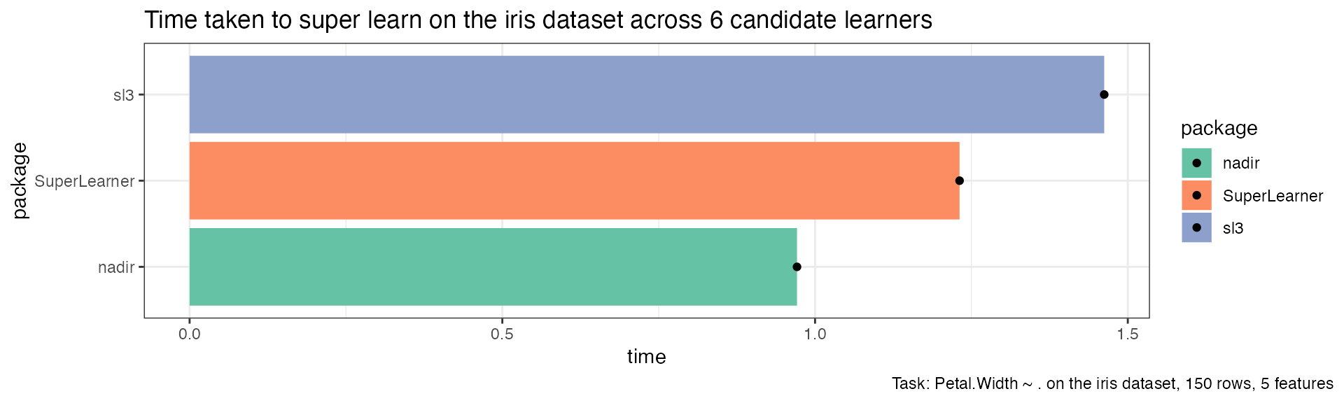
cv_timing <- data.frame(
  package = c('nadir', 'sl3', 'SuperLearner'),
  time = c(
    iris_nadir_cv_sl_benchmark[[3]], # user time
    iris_sl3_cv_sl_benchmark[[3]],
    iris_SuperLearner_cv_sl_benchmark[[3]])
)
cv_timing |>
  dplyr::mutate(package = forcats::fct_reorder(package, time)) |>
  ggplot(aes(x = time, y = package, fill = package)) +
  geom_col() +
  geom_point() +
  scale_fill_brewer(palette = 'Set2') +
  theme_bw() +
  ggtitle("Elapsed time taken to run cross-validated super learner on the iris dataset across 6 candidate learners",
          "Elapsed time (as opposed to user or system time) shows the amount of time experienced by the user.") +
  labs(caption = "Task: Petal.Width ~ . on the iris dataset, 150 rows, 5 features") +
  theme(plot.caption.position = 'plot')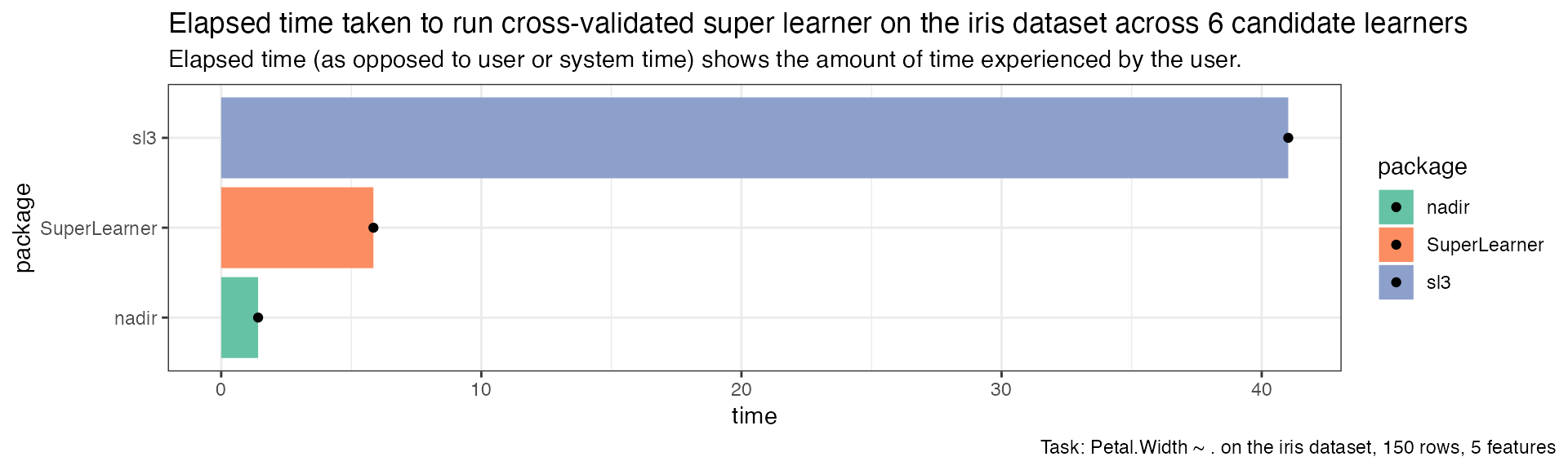
penguins data (16.8 KB)
penguins <- palmerpenguins::penguins
penguins <- penguins[complete.cases(penguins),]

flipper_length_formula <-
  flipper_length_mm ~ species + island + bill_length_mm +
    bill_depth_mm + body_mass_g + sex
nadir on penguins data (16.8 KB)
penguins_nadir_sl_benchmark <- microbenchmark(
  times = 10,
  nadir = {
    nadir::super_learner(
      data = penguins,
      formula = flipper_length_formula,
      learners = list(lnr_mean, lnr_lm, lnr_rf, lnr_earth, lnr_glmnet, lnr_xgboost)
    )
  }
)
penguins_nadir_sl_benchmark
#> Unit: seconds
#>   expr      min       lq     mean   median       uq      max neval
#>  nadir 1.157808 1.192269 1.290731 1.218286 1.309779 1.728092    10

penguins_nadir_cv_sl_benchmark <- system.time({
  cv_super_learner(
    data = penguins,
    formula = flipper_length_formula,
    learners = list(lnr_mean, lnr_lm, lnr_rf, lnr_earth, lnr_glmnet, lnr_xgboost)
  )
})
#> The loss_metric is being inferred based on the outcome_type=continuous -> using CV-MSE
penguins_nadir_cv_sl_benchmark
#>    user  system elapsed
#>   7.037   1.595   2.599
sl3 on penguins data (16.8 KB)
task <- make_sl3_Task(
  data = penguins,
  outcome = "flipper_length_mm",
  covariates = c("species",
                 "island",
                 "bill_length_mm",
                 "bill_depth_mm",
                 "body_mass_g",
                 "sex")
)

lrn_mean <- Lrnr_mean$new()
lrn_lm <- Lrnr_glm$new()
lrn_rf <- Lrnr_randomForest$new()
lrn_earth <- Lrnr_earth$new()
lrn_glmnet <- Lrnr_glmnet$new()
lrn_xgboost <- Lrnr_xgboost$new()

stack <- Stack$new(lrn_mean, lrn_lm, lrn_rf, lrn_earth, lrn_glmnet, lrn_xgboost)

sl <- Lrnr_sl$new(learners = stack, metalearner = Lrnr_nnls$new(),
                  cv_control = list(V = 5))

penguins_sl3_sl_benchmark <- microbenchmark::microbenchmark(
  times = 10,
  list(
    sl3 = { sl_fit <- sl$train(task = task) }
  )
)
penguins_sl3_sl_benchmark
#> Unit: seconds
#>                                                 expr      min       lq     mean
#>  list(sl3 = {     sl_fit <- sl$train(task = task) }) 1.314009 1.465803 2.642716
#>    median       uq      max neval
#>  1.640787 1.831675 9.482718    10


sl_fit <- sl$train(task = task)
penguins_sl3_cv_sl_benchmark <- system.time({
  sl3_cv = { cv_sl(lrnr_sl = sl_fit, eval_fun = loss_squared_error) }
})
#> [1] "Cross-validated risk:"
#> Key: <learner>
#>                                    learner       MSE        se   fold_sd
#>                                     <fctr>     <num>     <num>     <num>
#> 1:                               Lrnr_mean 196.47868 10.979336 33.704733
#> 2:                           Lrnr_glm_TRUE  28.08063  2.496742  6.675033
#> 3:            Lrnr_randomForest_500_TRUE_5  28.82479  2.349832  5.264787
#> 4:         Lrnr_earth_2_3_backward_0_1_0_0  29.00131  2.650027  5.636709
#> 5: Lrnr_glmnet_NULL_deviance_10_1_100_TRUE  28.39991  2.504920  6.139148
#> 6:                       Lrnr_xgboost_20_1  32.54006  2.627296  6.469929
#> 7:                            SuperLearner  19.35342  1.825590  6.853104
#>    fold_min_MSE fold_max_MSE
#>           <num>        <num>
#> 1:    139.88804    238.52211
#> 2:     16.23283     36.93534
#> 3:     17.60123     36.40382
#> 4:     21.20477     37.72809
#> 5:     19.34574     37.51000
#> 6:     21.36498     42.66572
#> 7:     11.12754     35.96351
penguins_sl3_cv_sl_benchmark
#>    user  system elapsed
#>  38.712  48.137  44.837
SuperLearner on penguins (16.8 KB)
data
sl_lib = c(
  "SL.mean", "SL.lm", "SL.randomForest", "SL.earth", "SL.glmnet", "SL.xgboost")

penguins_SuperLearner_sl_benchmark <- microbenchmark::microbenchmark(
  times = 10,
  list(SuperLearner = {
    mcSuperLearner(Y = penguins$flipper_length_mm,
                   X = penguins[, c("species",
                                    "island",
                                    "bill_length_mm",
                                    "bill_depth_mm",
                                    "body_mass_g",
                                    "sex")],
                 SL.library = sl_lib,
                 cvControl = list(V = 5))
  }
  )
)
penguins_SuperLearner_sl_benchmark
#> Unit: seconds
#>                                                                                                                                                                                                                                              expr
#>  list(SuperLearner = {     mcSuperLearner(Y = penguins$flipper_length_mm, X = penguins[,          c("species", "island", "bill_length_mm", "bill_depth_mm",              "body_mass_g", "sex")], SL.library = sl_lib, cvControl = list(V = 5)) })
#>       min       lq     mean   median       uq      max neval
#>  2.112144 2.154183 2.174983 2.175506 2.202207 2.224516    10

num_cores = RhpcBLASctl::get_num_cores()

penguins_SuperLearner_cv_sl_benchmark <- system.time({
  CV.SuperLearner(
    Y = penguins$flipper_length_mm,
    X = penguins[, c("species",
                     "island",
                     "bill_length_mm",
                     "bill_depth_mm",
                     "body_mass_g",
                     "sex")],
    SL.library = sl_lib,
    parallel = 'multicore',
    V = 5)
})
penguins_SuperLearner_cv_sl_benchmark
#>    user  system elapsed
#>   8.211   0.295  12.642
Visual comparison
sl_timing <- data.frame(
  package = c('nadir', 'sl3', 'SuperLearner'),
  time = c(mean(penguins_nadir_sl_benchmark$time) / 1e9, # convert nanoseconds to seconds
           mean(penguins_sl3_sl_benchmark$time) / 1e9,
           mean(penguins_SuperLearner_sl_benchmark$time) / 1e9)
)

ggplot(sl_timing, aes(x = time, y = package, fill = package)) +
  geom_col() +
  geom_point() +
  scale_fill_brewer(palette = 'Set2') +
  theme_bw() +
  ggtitle("Time taken to super learn on the penguins dataset across 6 candidate learners") +
  labs(caption = "Task: flipper_length_mm ~ . on the penguins dataset, 333 rows, 8 features") +
  theme(plot.caption.position = 'plot')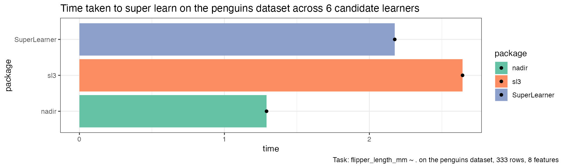
cv_timing <- data.frame(
  package = c('nadir', 'sl3', 'SuperLearner'),
  time = c(
    penguins_nadir_cv_sl_benchmark[[3]], # user time
    penguins_sl3_cv_sl_benchmark[[3]],
    penguins_SuperLearner_cv_sl_benchmark[[3]])
)
cv_timing |>
  dplyr::mutate(package = forcats::fct_reorder(package, time)) |>
  ggplot(aes(x = time, y = package, fill = package)) +
  geom_col() +
  geom_point() +
  scale_fill_brewer(palette = 'Set2') +
  theme_bw() +
  ggtitle("Elapsed time taken to run cross-validated super learner on the penguins dataset across 6 candidate learners",
          "Elapsed time (as opposed to user or system time) shows the amount of time experienced by the user.") +
  labs(caption = "Task: flipper_length_mm ~ . on the penguins dataset, 333 rows, 8 features") +
  theme(plot.caption.position = 'plot')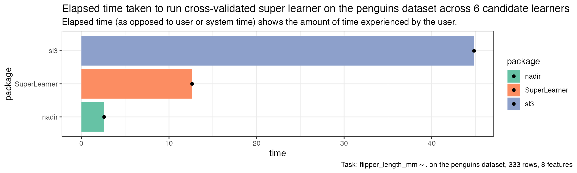
tornados data (2.8 MB)
# recommendations from here for dealing with large data
# in future multicore setup https://github.com/satijalab/seurat/issues/1845
options(future.globals.maxSize = 8000 * 1024^2)

tuesdata <- tidytuesdayR::tt_load('2023-05-16')
tornados <- tuesdata$tornados
tornados <- tornados[,c('yr', 'mo', 'dy', 'mag', 'st', 'inj', 'fat', 'loss')]
tornados <- tornados[complete.cases(tornados),]

# these states appear only very infrequently, like 2 and 1 times respectively — DC and Alaska
tornados <- tornados |> dplyr::filter(!st %in% c('DC', 'AK'))

tornado_formula <- inj ~ yr + mo + mag + fat + st + loss
nadir on tornados data (2.8 MB)
tornados_nadir_sl_benchmark <- system.time({
  super_learner(
    data = tornados,
    formula = tornado_formula,
    learners = list(lnr_mean, lnr_lm, lnr_rf, lnr_earth, lnr_glmnet, lnr_xgboost),
    cv_schema = cv_character_and_factors_schema
  )
})
tornados_nadir_sl_benchmark
sl3 on tornados data (2.8 MB)
task <- make_sl3_Task(
  data = tornados,
  outcome = "inj",
  covariates = c("yr", "mo", "dy", "mag",
                 "st", "fat", "loss")
)

lrn_mean <- Lrnr_mean$new()
lrn_lm <- Lrnr_glm$new()
lrn_rf <- Lrnr_randomForest$new()
lrn_earth <- Lrnr_earth$new()
lrn_glmnet <- Lrnr_glmnet$new()
lrn_xgboost <- Lrnr_xgboost$new()

stack <- Stack$new(lrn_mean, lrn_lm, lrn_rf, lrn_earth, lrn_glmnet, lrn_xgboost)

sl <- Lrnr_sl$new(learners = stack, metalearner = Lrnr_nnls$new(),
                  cv_control = list(V = 5))

tornados_sl3_sl_benchmark <- system.time({
  sl_fit <- sl$train(task = task)
})
tornados_sl3_sl_benchmark
SuperLearner on tornados data (2.8
MB)
Unfortunately we were unable to get results from the
SuperLearner package with the tornados dataset, as it
produced an obscure error and little to no guidance on how to debug the
error is presently available.
sl_lib = c(
  "SL.mean", "SL.lm", "SL.randomForest", "SL.earth", "SL.glmnet", "SL.xgboost")

tornados_SuperLearner_sl_benchmark <- system.time({
    mcSuperLearner(Y = tornados$inj,
                   X = tornados[, c("yr", "mo", "dy", "mag",
                 "st", "fat", "loss")],
                 SL.library = sl_lib,
                 cvControl = list(V = 5))
  })
error produced by SuperLearner on the tornados
dataset
Visualizing Results
sl_timing <- data.frame(
  package = c('nadir', 'sl3', 'SuperLearner'),
  time = c(tornados_nadir_sl_benchmark[[3]],
    tornados_sl3_sl_benchmark[[3]],
    NA))

sl_timing |>
  ggplot(aes(y = package, x = time, fill = package)) +
  geom_col() +
  geom_point() +
  xlab("Seconds") +
  geom_text(
    data = data.frame(package = 'SuperLearner', label = 'failed to run', time = 200),
    mapping = aes(label = label)) +
  theme_bw() +
  scale_fill_brewer(palette = 'Set2') +
  ggtitle("Time taken to super learn on the tornados dataset across 6 candidate learners") +
  labs(caption = "Task: inj ~ . on the tornados dataset, 41,514 rows, 8 features, 2.8 MB") +
  theme(plot.caption.position = 'plot', panel.grid.major.y = element_blank())
timing results with the tornados dataset