Binary and Multiclass Outcomes

library(nadir)

I want to use super_learner() for binary outcomes.

We’ll use the Boston dataset and create a binary outcome for our regression problem.

And of course, we’ll train a super_learner() to these binary outcomes.
To handle binary outcomes, we need to adjust the method for determining weights. This is because we don’t want to use the default mse() loss function, but instead we should to rely on using the negative log likelihood loss on the held-out data. To do this appropriately in the context of binary data, we use the determine_weights_for_binary_outcomes() function provided by nadir.

data('Boston', package = 'MASS')

# create a binary outcome to predict
Boston$high_crime <- as.integer(Boston$crim > mean(Boston$crim))
data <- Boston |> dplyr::select(-crim)

# train a super learner on a binary outcome
trained_binary_super_learner <- super_learner(
  data = data,
  formula = high_crime ~ nox + rm + age + tax + ptratio,
  learners = list(
    logistic = lnr_logistic, # the same as a lnr_glm with extra_learner_args 
                             # set to list(family = binomial(link = 'logit'))
                             # for that learner
    rf = lnr_rf_binary,  # random forest
    lm = lnr_lm), # linear probability model
  outcome_type = 'binary',
  verbose = TRUE
)

# let's take a look at the learned weights
trained_binary_super_learner$learner_weights
#>     logistic           rf           lm 
#> 1.000000e+00 2.691182e-16 4.748858e-20

# what are the predictions? you can think of them as \hat{P}(Y = 1 | X).
# i.e., predictions of P(Y = 1) given X where Y and X are the left & right hand
# side of your regression formula(s)
head(trained_binary_super_learner$sl_predict(data))
#>            1            2            3            4            5            6 
#> 2.772297e-05 1.034418e-05 5.749397e-06 2.472188e-06 3.237557e-06 3.784687e-06

# classification table
data.frame(
  truth = data$high_crim, 
  prediction = round(trained_binary_super_learner$sl_predict(data))) |> 
  dplyr::group_by(truth, prediction) |> 
  dplyr::count() |> 
  ggplot2::ggplot(mapping = ggplot2::aes(y = truth, x = prediction, fill = n, label = n)) + 
  ggplot2::geom_tile() + 
  ggplot2::geom_label(fill = 'white', alpha = .7) + 
  ggplot2::scale_fill_distiller(palette = 'Oranges', direction = 1) + 
  ggplot2::scale_x_continuous(breaks = c(0, 1)) + 
  ggplot2::scale_y_continuous(breaks = c(0, 1)) + 
  ggplot2::xlab("super_learner() prediction") + 
  ggplot2::theme_minimal() + 
  ggplot2::theme(legend.position = 'none') + 
  ggplot2::ggtitle("Classification Table")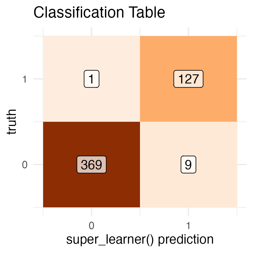

data.frame(
  truth = data$high_crim, 
  predicted_pr_of_1 = trained_binary_super_learner$sl_predict(data)) |> 
  ggplot2::ggplot(mapping = ggplot2::aes(x = predicted_pr_of_1)) + 
  ggplot2::geom_histogram() + 
  ggplot2::facet_grid(truth ~ ., labeller = ggplot2::labeller(truth = ~ paste0('truth: ', .))) + 
  ggplot2::theme_bw() + 
  ggplot2::theme(panel.grid.minor = ggplot2::element_blank()) + 
  ggplot2::xlab(bquote(paste("super_learner() predictions, ", hat(bold(P)), '(Y = 1)'))) + 
  ggplot2::ggtitle("Classification Task") 
#> `stat_bin()` using `bins = 30`. Pick better value with `binwidth`.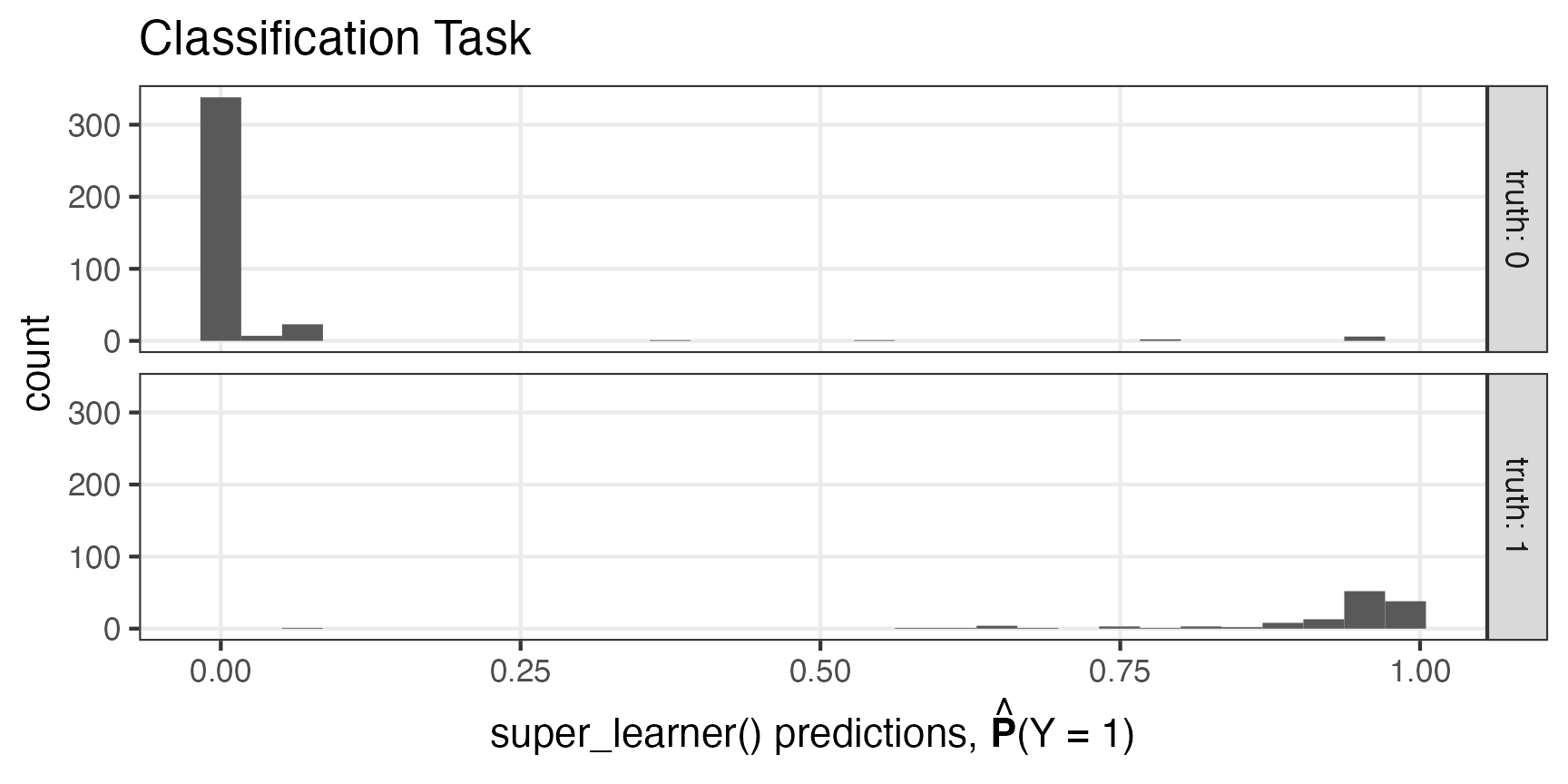

An important thing to know about constructing learners for the binary outcome context is that determine_weights_for_binary_outcomes() requires that the outputs of the learners on newdata are predictions for the outcome being equal to 1.

Multiclass Regression, i.e., Multinomial Regression

Earlier we covered binary classification — now we turn to classification problems where the dependent variable is one of a discrete number of unique levels.

nadir includes two learners that are designed for such multiclass regression problems: lnr_multinomial_vglm and lnr_multinomial_nnet.

We can perform super learning with them and a classification problem like that of classifying the penguins’ species in the palmerpenguins dataset.

library(palmerpenguins)

df <- penguins[complete.cases(penguins),]

sl_learned_model <- super_learner(
  data = df,
  formulas = list(
    .default = species ~ flipper_length_mm + bill_depth_mm,
    nnet2 = species ~ poly(flipper_length_mm, 2) + poly(bill_depth_mm, 2) + body_mass_g,
    nnet3 = species ~ flipper_length_mm * bill_depth_mm + island
    ),
  learners = list(
    nnet1 = lnr_multinomial_nnet,
    nnet2 = lnr_multinomial_nnet,
    nnet3 = lnr_multinomial_nnet,
    vglm = lnr_multinomial_vglm
    ),
  outcome_type = 'multiclass',
  verbose = TRUE)


compare_learners(sl_learned_model, loss_metric = negative_log_loss)
#> # A tibble: 1 × 4
#>   nnet1 nnet2 nnet3  vglm
#>   <dbl> <dbl> <dbl> <dbl>
#> 1  120.  119.  156.  120.

round(sl_learned_model$learner_weights, 3)
#> nnet1 nnet2 nnet3  vglm 
#> 0.000 0.000 0.956 0.044