Doubly Robust Estimation • nadir

One of the central tasks of causal inference is the estimation of average treatment effects. There are many approaches to doing this, but one of particular importance is that of doubly robust estimation.

The following article provides example code for how to create a doubly robust estimator of an average treatment effect (ATE) using nadir::super_learner().

Background

For some useful references on doubly robust estimation, we refer the curious reader to:

Kang, J. D. Y., & Schafer, J. L. (2007). Demystifying Double Robustness: A Comparison of Alternative Strategies for Estimating a Population Mean from Incomplete Data. Statistical Science, 22(4). https://doi.org/10.1214/07-sts227
Fine Point 13.2 and Technical Point 13.2 of Hernán MA, Robins JM (2020). Causal Inference: What If. Boca Raton: Chapman & Hall/CRC https://miguelhernan.org/whatifbook
Funk, M. J., Westreich, D., Wiesen, C., Stürmer, T., Brookhart, M. A., & Davidian, M. (2011). Doubly Robust Estimation of Causal Effects. American Journal of Epidemiology, 173(7), 761–767. https://doi.org/10.1093/aje/kwq439
Bang, H., & Robins, J. M. (2005). Doubly Robust Estimation in Missing Data and Causal Inference Models. Biometrics, 61(4), 962–973. https://doi.org/10.1111/j.1541-0420.2005.00377.x
Zivich, P. N., & Breskin, A. (2021). Machine Learning for Causal Inference: On the Use of Cross-fit Estimators. Epidemiology, 32(3), 393–401. https://doi.org/10.1097/ede.0000000000001332

For a very informal, but introductory explanation, the StitchFix tech blog Multithreaded has a very nice article here:

Nettiksimmons, J. & Davies, M. (2021). Gimme a robust estimator - and make it a double! https://multithreaded.stitchfix.com/blog/2021/07/23/double-robust-estimator/

In particular, the following paragraph from Zivich and Breskin nicely summarizes why it is important to use a doubly robust estimator if using machine learning algorithms and/or cross-fit estimators like those from nadir::super_learner():

The need for doubly-robust estimators with cross-fitting when using data-adaptive machine learning for nuisance function estimation arises from two terms in the Von Mises expansion of the estimator. The first term, which is described by an empirical process term in the expansion, can be controlled by either restricting the complexity of the nuisance models (e.g., by requiring them to be in the Donsker class) or through cross-fitting. Because it can be difficult or impossible to verify that a given machine learning method is in the Donsker class, cross-fitting provides a simple and attractive alternative. The second term is the second-order remainder, and it converges to zero as the sample size increases. For valid inference, it is desirable for this remainder term to converge as a function of n−1/2, referred to as as root-n convergence. Convergence rates are not a computational issue, but rather a feature of the estimator itself. Unfortunately, data-adaptive algorithms often have slower convergence rates as a result of their flexibility. However, because the second-order remainder term of doubly-robust estimators is the product of the approximation errors of the treatment and outcome nuisance models, doubly-robust estimators only require that the product of the convergence rates for nuisance models be n−1/2. To summarize, cross-fitting permits the use of highly complex nuisance models, while doubly-robust estimators permit the use of slowly converging nuisance models. Used together, these approaches allow one to use a wide class of data-adaptive machine learning methods to estimate causal effects.

Constructing an Example Dataset

We will create a synthetic dataset in which we model the effect of an active drug (treatment) vs. placebo (control) on a generic health outcome. Additionally, in our simulated data, the treatment assignment mechanism to the drug arm will not be completely random, but rather dependent on some observed covariates (for example, age and income). This could reflect either an observational setting where participants self-selected into the treatment arms, or a randomized setting, but where the assignment into arms was designed by investigators to (stochastically) rely on age and income.

library(dplyr)
library(tibble)
library(ggplot2)
library(patchwork)
library(nadir)

sample_size <- 5000 # sample size for the simulation dataset

# the simulation dataset has the following properties: 
#   the A->Y is confounded by the L->A and L->Y pathways; 
# 
#   Y_observed is the "coarsened" or observed one of the two 
#   potential outcomes Y(0) and Y(1). 
# 
#   Y(0) and Y(1) are constructed as the output of a baseline 
#   mean model given L1 and L2 (mu) and a heterogeneous treatment
#   effect (tau), again given L1 and L2 
df <- 
  tibble::tibble(
    # ages are taken to be between 30 and 50 
    L1_age = sample(x = seq(30, 50), size = sample_size, replace = TRUE),
    # household income is centered around $35,000, with a floor of $5,000 
    L2_income = rlnorm(n=sample_size, meanlog = log(30000), sdlog = log(3)) + 5000,
    
    # Treatment mechanism: logit depends on age and (log) income
    A_treatment = rbinom(
      n = sample_size,
      size = 1,
      prob = plogis(-6 + 0.6 * (L1_age - 40) + 4 * log(L2_income / 40000))
    ),
    
    # Outcome model components: baseline mu(L) and heterogeneous effect tau(L)
    mu  = 50 + 0.15 * (L1_age - 40) - 2.5 * log(L2_income / 40000),
    tau =  4 + 0.05 * (50 - L1_age) + 1.2 * log(L2_income / 40000),
  
    # Potential outcomes and observed outcome
    `Y(0)` = rnorm(sample_size, mean = mu,          sd = 1),
    `Y(1)` = rnorm(sample_size, mean = mu + tau,    sd = 1),
    Y_observed = dplyr::if_else(A_treatment == 1L, `Y(1)`, `Y(0)`)) |> 
  dplyr::select(-mu, -tau)

Visualizing Confounding in the Dataset

Below we visualize how the treatment-assignment and treatment effect on the outcome are confounded by the age and income covariates.

Intuitively, the way to understand the problem this confounding poses to estimating an average treatment effect is as follows:

Under a completely randomized regime, we’d like to be able to simply compare the treated to the placebo arm in their outcomes.
However, the people in the treated arm are systematically different (in a distributional sense) from the people in the placebo arm. They are higher in income and age, on average.
As a result, any good estimator for the average treatment effect should take this systematic difference into account.

default_theme <- theme_bw()

p1 <- ggplot(df, aes(x = L1_age, y = A_treatment)) + 
  geom_jitter(height = 0.025, width = 0.25, alpha = 0.1) + 
  stat_smooth(formula = "y ~ x", method = "glm", 
                method.args = list(family="binomial"), se = FALSE) + 
  default_theme + 
  ggtitle(expression(Age %->% Treatment)) 

p2 <- ggplot(df, aes(x = L2_income, y = A_treatment)) + 
  geom_jitter(height = 0.025, width = 0.25, alpha = 0.1) + 
  stat_smooth(formula = "y ~ x", method = "glm", 
                method.args = list(family="binomial"), se = FALSE) + 
  default_theme + 
  scale_x_log10(labels = scales::dollar_format()) + 
  ggtitle(expression(Income %->% Treatment))

p3 <- ggplot(df, aes(x = L1_age, y = Y_observed)) + 
  geom_jitter(width = 0.25, height = 0.025, alpha = 0.1) + 
  geom_smooth(se = FALSE) + 
  default_theme + 
  ggtitle(expression(Age %->% Outcome))

p4 <- ggplot(df, aes(x = L2_income, y = Y_observed)) + 
  geom_point(alpha = 0.1) + 
  geom_smooth(se = FALSE) + 
  default_theme + 
  scale_x_log10(labels = scales::dollar_format()) + 
  ggtitle(expression(Income %->% Outcome))

patchwork <- { p1 | p2 } / { p3 | p4 } 

patchwork + plot_annotation(
  title = "Evidence of Confounding",
  subtitle =  
                    expression(paste("The following four relationships are visualized: ", list(L[1], L[2] %->% A, L[1], L[2] %->% Y))),
  theme = theme(plot.title = element_text(size = 18))
) & 
  theme(text = element_text(size = 10))
#> `geom_smooth()` using method = 'gam' and formula = 'y ~ s(x, bs = "cs")'
#> `geom_smooth()` using method = 'gam' and formula = 'y ~ s(x, bs = "cs")'

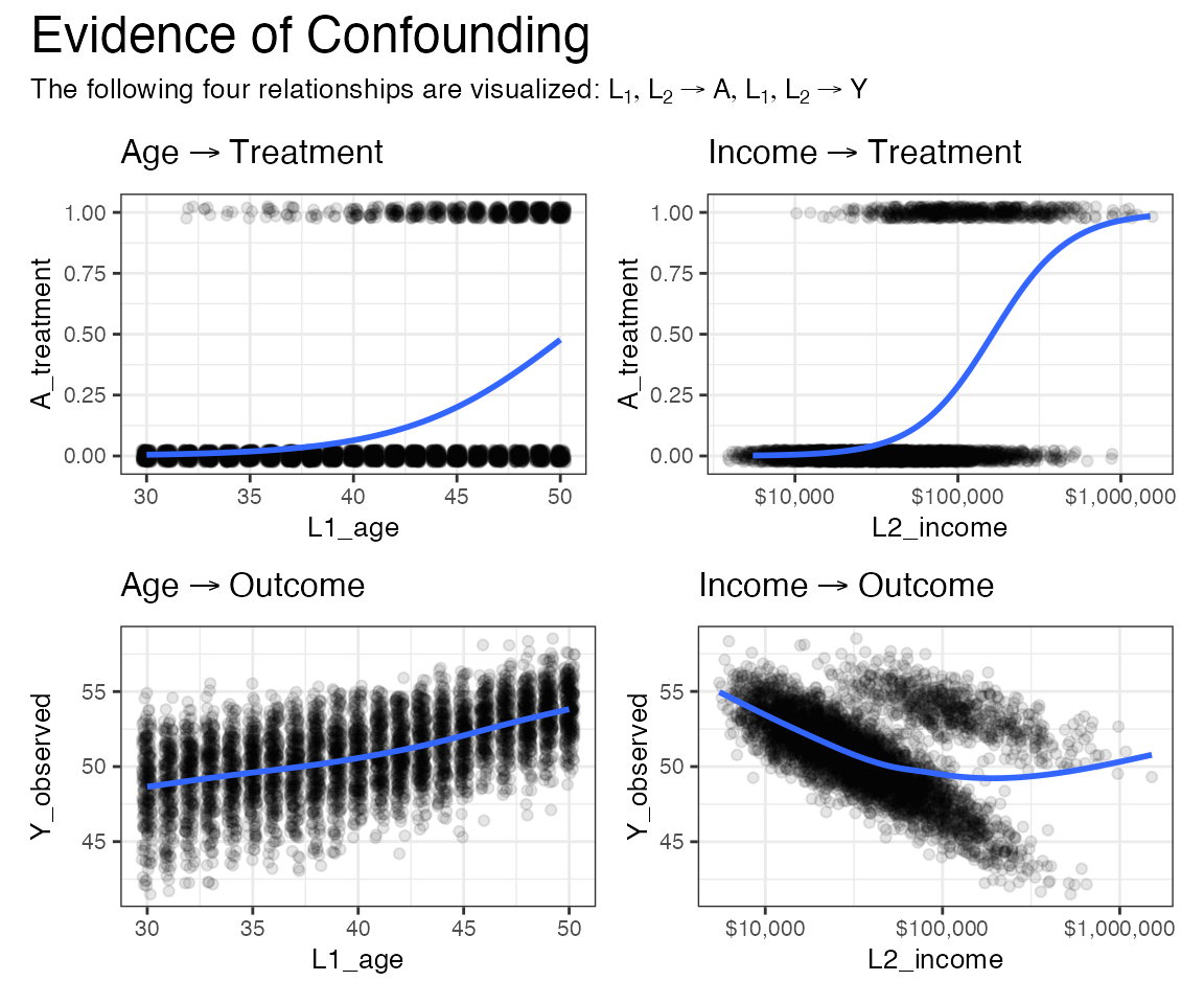
Determine the True Average Treatment Effect

Since the data are simulated including both poptential outcomes $Y(1)$ and $Y(0)$ , we are able to obtain the average treatment effect for this population as a simple average of the individual treatment effects. Normally, this is not possible in the real world, because we cannot assign both treatment and placebo to the same individuals in order to observe both potential outcomes.

# the true average treatment effect
true_ate <- mean(df$`Y(1)` - df$`Y(0)`)
print(paste0("True ATE: ", round(true_ate, 2)))
#> [1] "True ATE: 4.4"

# visualize the individual treatment effects
ggplot(df, aes(x = `Y(1)` - `Y(0)`)) +
  geom_histogram(fill = 'cadetblue', alpha = 0.4) +
  geom_vline(xintercept = true_ate, color = 'firebrick') +
  default_theme +
  xlab("Individual Treatment Effect") +
  ggtitle(
    "Histogram of the Individual Treatment Effects",
    subtitle = paste0(
      "We can only know these because this is a simulation.  The ATE is shown by the red vertical line."))
#> `stat_bin()` using `bins = 30`. Pick better value with `binwidth`.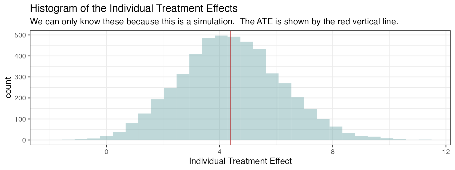

So this number, 4.4, is what we’re looking to estimate with our doubly robust code below, and without knowledge of Y(1) and Y(0) but instead only of Y_observed.

Fitting the Outcome and Propensity Score Models

As a reminder, the outcome model refers to the model of the outcome given the treatment received and covariates, while the propensity score refers to the probability of receiving treatment given the covariates.

In mathematical notation, we denote these as

$m_A(L) \equiv \mathbb{E}\left[ Y \mid A, L\right],$ and $\pi(L) \equiv \mathbb{P}(A = 1 \mid L).$

The above refer to the true outcome model and propensity score models, but when we estimate them from the data using an algorithm, we refer to the estimated models as $\hat{m}_A(L)$ and $\hat{\pi}(L)$ .

Note that in the real world, we don’t get to see both $Y(1)$ and $Y(0)$ – we only get to see the observed outcome, which is $Y = A Y(1) + (1-A) Y(0)$ . As such, we’ll drop the values Y(1) and Y(0) from the dataset so we don’t risk accidentally making any use of them in our estimation procedure.

df <- df |> dplyr::select(-c(`Y(1)`, `Y(0)`))

Now we’re ready to fit outcome and propensity score models to the data. To be as flexible as possible, we will use nadir::super_learner() with a variety of different learners.

outcome_model <- super_learner(
  data = df, 
  formulas = list(
    .default = Y_observed ~ L1_age + L2_income + A_treatment,
    gam = Y_observed ~ s(L1_age, L2_income) + A_treatment),
  learners = list(
    mean = lnr_mean,
    lm = lnr_lm,
    earth = lnr_earth,
    rf = lnr_rf,
    gam = lnr_gam,
    hal = lnr_hal
    ),
  verbose = TRUE)

propensity_model <- super_learner(
  data = df, 
  formulas = list(
    .default = A_treatment ~ L1_age + L2_income,
    gam = A_treatment ~ s(L1_age, L2_income)),
  learners = list(
    mean = lnr_mean,
    logistic = lnr_logistic,
    rf = lnr_rf_binary,
    earth = lnr_earth,
    xgboost = lnr_xgboost,
    gam = lnr_gam,
    hal = lnr_hal),
  extra_learner_args = list(
    earth = list(glm = list(family='binomial')),
    xgboost = list(param = list(objective = 'binary:logistic')),
    gam = list(family = binomial),
    hal = list(family = 'binomial')
  ),
  outcome_type = 'binary',
  determine_super_learner_weights = determine_weights_for_binary_outcomes,
  verbose = TRUE
)

There are fit diagnostics available that allow us to see which learners were favored, and how they performed:

# learner weights 
round(outcome_model$learner_weights, 2)
#>  mean    lm earth    rf   gam   hal 
#>  0.00  0.00  0.02  0.00  0.52  0.46
round(propensity_model$learner_weights, 2)
#>     mean logistic       rf    earth  xgboost      gam      hal 
#>     0.00     0.03     0.07     0.00     0.09     0.76     0.05

# compare learners by their loss metric
compare_learners(outcome_model)
#> Inferring the loss metric for learner comparison based on the outcome type:
#> outcome_type=continuous -> using mean squared error
#> # A tibble: 1 × 6
#>    mean    lm earth    rf   gam   hal
#>   <dbl> <dbl> <dbl> <dbl> <dbl> <dbl>
#> 1  7.15  3.16  1.13  1.73  1.10  1.12
compare_learners(propensity_model)
#> Inferring the loss metric for learner comparison based on the outcome type:
#> outcome_type=binary -> using negative log loss
#> # A tibble: 1 × 7
#>    mean logistic    rf earth xgboost   gam   hal
#>   <dbl>    <dbl> <dbl> <dbl>   <dbl> <dbl> <dbl>
#> 1 1957.     811.   Inf  903.   1019.  632.  651.

Doubly Robust Estimation and Inference

Now that we’ve fit our outcome model $\hat{m}_A(L)$ and our propensity score model $\hat{\pi}(L)$ , we can proceed with constructing a doubly robust estimate of the average treatment effect.

The doubly robust estimator has the following form:

$\hat \theta_{\text{DR}} = \frac{1}{n} \sum_{i=1}^n \left\{ \left( \hat m_1(L_i) + \frac{A_i}{\hat \pi(L_i)} (Y_i - \hat m_1(L_i))\right) - \left( \hat m_0(L_i) + \frac{1-A_i}{1-\hat \pi(L_i)}(Y_i - \hat m_0(L_i)) \right) \right\}.$

$\hat{\theta}_{\text{DR}}$ is an asymptotically linear estimator, and the above representation of it can be viewed as a sample average of independent and identically distributed terms. The result is that we can use the theory of asymptotic linearity and influence functions to construct asymptotically valid confidence intervals.

Some useful references on influence function based inference are

Hines, O., Dukes, O., Diaz-Ordaz, K., & Vansteelandt, S. (2022). Demystifying Statistical Learning Based on Efficient Influence Functions. The American Statistician, 76(3), 292–304. https://doi.org/10.1080/00031305.2021.2021984
Kennedy, E. H. (2022). Semiparametric doubly robust targeted double machine learning: a review (Version 2). arXiv. https://doi.org/10.48550/ARXIV.2203.06469
Fisher, A., & Kennedy, E. H. (2020). Visually Communicating and Teaching Intuition for Influence Functions. The American Statistician, 75(2), 162–172. https://doi.org/10.1080/00031305.2020.1717620

A <- df$A_treatment
Y <- df$Y_observed 

# get components of propensity scores
pi_hat_of_L <- propensity_model$sl_predictor(df)
one_minus_pi_hat_of_L <- 1-pi_hat_of_L

# get outcome predictions
m_of_0_exposure_and_L <-
  outcome_model$sl_predictor({
    df |> mutate(A_treatment = 0)
  })
m_of_1_exposure_and_L <-
  outcome_model$sl_predictor({
    df |> mutate(A_treatment = 1)
  })


# the following expression is the doubly robust estimator for the average
# treatment effect in the presence of confounders 
ATE_AIPW <- 
  mean(
    (m_of_1_exposure_and_L + (Y - m_of_1_exposure_and_L) / pi_hat_of_L * A) - 
      (m_of_0_exposure_and_L + (Y - m_of_0_exposure_and_L) / one_minus_pi_hat_of_L * (1-A))
  )

# in order to conduct inference, we can use the influence curve of the 
# estimator and take its variance divided by n
IF <-
  A * Y / pi_hat_of_L - 
  (A - pi_hat_of_L) / pi_hat_of_L * m_of_1_exposure_and_L -
  (1 - A) * Y / one_minus_pi_hat_of_L - 
  ((1 - A) - one_minus_pi_hat_of_L) / one_minus_pi_hat_of_L * m_of_0_exposure_and_L - 
  ATE_AIPW # this is the centered influence function

ATE_AIPW_variance_estimate <- var(IF)/nrow(df)

ATE_ConfidenceIntervals <- ATE_AIPW + qnorm(c(0.025, 0.975)) * sqrt(ATE_AIPW_variance_estimate)
formatted_CI <-
  paste0("(", paste0(round(ATE_ConfidenceIntervals, 2), collapse = ', '),
         ")")

cat(paste0(
  "ATE Estimate: ", round(ATE_AIPW, 2), "\n",
  "Confidence Intervals: ", formatted_CI, "\n"))
#> ATE Estimate: 4.35
#> Confidence Intervals: (2.92, 5.79)

Conclusions

It looks like our estimate 4.35 is quite close to the true value, 4.4, which is great! Moreover, the truth easily lies within the confidence interval produced (2.92, 5.79).

What is truly remarkable about this approach, as you can read about in the references listed throughout this article, is that by cross-fitting our nuisance models (as in, via nadir::super_learner()) and using a doubly robust estimator, we are able to avoid problems related to the curse of dimensionality in machine learning algorithms and are able to produce consistent estimates of causal parameters with asymptotically valid confidence intervals under relatively mild assumptions.

If you want to keep going with nadir::super_learner() for causal inference, natural subsequent directions are to use it with other causal parameters besides the ATE and/or in other efficient inferential paradigms like Targeted Learning, in a one-step estimation, or sequentially doubly robust estimation.