library(nadir)
#> Registered S3 method overwritten by 'future':
#>   method               from
#>   all.equal.connection parallelly
library(ggplot2)
#> Warning: package 'ggplot2' was built under R version 4.3.3
Thinking about applications of the super learner algorithm to causal inference, one key application is through modeling the treatment/exposure mechanism.
In many cases, the treatment/exposure is continuous, necessitating the estimation of a “generalized” propensity score — generalized in the sense that the treatment/exposure is no longer binary but continuous, and hence our propensity score model is a probability density model for a continuous range of exposure values rather than just the probability of a binary treatment/no-treatment variable.
Here we demonstrate the application of
nadir::super_learner() in estimating such generalized
propensity scores.
The following examples are provided in the spirit of showing a myriad number of ways nadir can be used to tackle density estimation.
Basic Syntax for Fitting Density Models
To fit a conditional density model, we need a few things:
- a dataset
- to select the outcome, and predictor variables (which together define a formula)
- a collection of candidate learners
- and to use the negative log loss function in the super learner algorithm for choosing among the learners.
# specify our data and regression problem
# ---------------------------------------

# in order to build a weighting based estimator, we might fit a conditional
# density model of our continuous exposure
data("Boston", package = "MASS")

# we're going to regress the crime measurement variable in the Boston dataset
# on all the other variables.
#
# and we want to control for the following potential confounders (all other variables in the Boston dataset)
#
# so we want to regress crime on all the other variables in the Boston dataset
reg_formula <- crim ~ .


# specify a collection of candidate learners
# ------------------------------------------

# we'll use a normal error model with a linear conditional mean model,
# and random forest, ranger, lm, and earth with kernel bandwidth density() models for the
# error distribution

# nadir provides the helper function lnr_homoskedastic_density that can be used
# to build a homoskedastic density learner out of a given conditional mean learner.

lnr_rf_homoskedastic_density <- function(data, formula, ...) {
  lnr_homoskedastic_density(data, formula, mean_lnr = lnr_rf, ...)
}

lnr_ranger_homoskedastic_density <- function(data, formula, ...) {
  lnr_homoskedastic_density(data, formula, mean_lnr = lnr_ranger, ...)
}

lnr_lm_homoskedastic_density <- function(data, formula, ...) {
  lnr_homoskedastic_density(data, formula, mean_lnr = lnr_lm, ...)
}

lnr_earth_homoskedastic_density <- function(data, formula, ...) {
  lnr_homoskedastic_density(data, formula, mean_lnr = lnr_earth, ...)
}

# we recommend setting the sl_lnr_type attribute to avoid warnings from super_learner()
#
# this tells the super_learner() function that these learners are designed
# to work with density estimation problems.
#
# without this, users will see a friendly warning asking them if they're sure
# they want to use the given learners with the outcome_type = 'density'.
#
attr(lnr_rf_homoskedastic_density, 'sl_lnr_type') <- 'density'
attr(lnr_ranger_homoskedastic_density, 'sl_lnr_type') <- 'density'
attr(lnr_lm_homoskedastic_density, 'sl_lnr_type') <- 'density'
attr(lnr_earth_homoskedastic_density, 'sl_lnr_type') <- 'density'


# super learning:
# choosing weights for candidate learners and ensembling
# ======================================================

learned_sl_density_model <- super_learner(
  data = Boston,
  formula = reg_formula,
  learners = list(
    normal = lnr_lm_density,
    ranger = lnr_ranger_homoskedastic_density,
    earth = lnr_earth_homoskedastic_density,
    lm = lnr_lm_homoskedastic_density
    ),
  outcome_type = 'density',
  verbose = TRUE
)

# if you prefer not to code up the new learners as above, another way to perform
# the same super learning as above is to use the `extra_learner_args` option
# with named learners as follows:
#
# learned_sl_density_model <- super_learner(
#   data = Boston,
#   formula = reg_formula,
#   learners = list(
#     normal = lnr_lm,
#     ranger = lnr_homoskedastic_density,
#     earth = lnr_homoskedastic_density,
#     lm = lnr_lm_homoskedastic_density
#     ),
#   extra_learner_args = list(
#     ranger = list(mean_lnr = lnr_ranger),
#     earth = list(mean_lnr = lnr_earth),
#     lm = list(mean_lnr = lnr_lm)),
#   outcome_type = 'density',
#   verbose = TRUE
# )
#
# one reason it can be useful to create the learners explicitly is to be able to
# visualize and debug their behaviors individually.


# fit diagnostics
# ===============

# two things we might want to do with a fit super learner model are:
# 1) see how each candidate learner performed with regard to the specified loss
#    function
# 2) see the weights assigned to each learner (how favored they are in the final
#    ensemble model).
#
# to be able to see these diagnostics, it's important that super_learner() is
# run with vebose = TRUE otherwise these extra details are not stored in the
# output object.

# 1) compare the learners using negative log likelihood loss
compare_learners(learned_sl_density_model, loss_metric = negative_log_loss)
#> # A tibble: 1 × 4
#>   normal ranger earth    lm
#>    <dbl>  <dbl> <dbl> <dbl>
#> 1  1716.  1055. 1403. 1473.

# 2) see the weights given to each candidate learner
learned_sl_density_model$learner_weights
#>     normal     ranger      earth         lm
#> 0.07190413 0.87099445 0.02994368 0.02715774
Let’s validate that conditional density works the way it should
One test we can do to check that conditional density estimation is working correctly is that once we condition on a set of predictors, the produced probability density function should integrate to 1 – that is, its area under the curve should be equal to 1.
We show an example of a test here:
lm_density_predict <- lnr_lm_homoskedastic_density(Boston, reg_formula)

f_lm <- function(ys) {
  x <- Boston[1,]
  sapply(ys, function(y) {
    x[['crim']] <- y
    lm_density_predict(x)
  })
}

integrate(f_lm, min(Boston$crim) - sd(Boston$crim), max(Boston$crim) + sd(Boston$crim), subdivisions = 10000)
#> 0.981094 with absolute error < 6.9e-05


earth_density_predict <- lnr_earth_homoskedastic_density(Boston, reg_formula, density_args = list(bw = 30))

f_earth <- function(ys) {
  x <- Boston[1,]
  sapply(ys, function(y) {
    x[['crim']] <- y
    earth_density_predict(x)
  })
}
earth_density_predict(Boston[1,])
#> [1] 0.01315833

# we're looking for this number to be very close to 1:
integrate(f_earth, min(Boston$crim) - 10*sd(Boston$crim), max(Boston$crim) + 10*sd(Boston$crim))
#> 0.9987836 with absolute error < 5.4e-05


# sometimes if integrate() has trouble, it's useful to perform the integration by hand:
y_seq <- seq(min(Boston$crim) - 10*sd(Boston$crim), max(Boston$crim) + 10*sd(Boston$crim), length.out = 10000)
delta_y <- y_seq[2]-y_seq[1]
sum(f_earth(y_seq)*delta_y) # we're looking for this to be close to 1
#> [1] 0.9987911
Heteroskedastic Learners
lnr_earth_mean_glm_var_heteroskedastic_density <- function(data, formula, ...) {
  lnr_heteroskedastic_density(
    data,
    formula,
    mean_lnr = lnr_earth,
    var_lnr = lnr_lm,
    density_args = list(bw=5),
    ...
  )
}

Boston$log_crim <- log(Boston$crim)

earth_mean_glm_var_heteroskedastic_predict <-
  lnr_earth_mean_glm_var_heteroskedastic_density(Boston[,-1], log_crim ~ medv)

earth_mean_glm_var_heteroskedastic_predict(Boston[1,])
#> [1] 0.07019618

f_earth_glm <- function(ys) {
  x <- Boston[2,]
  sapply(ys, function(y) {
    x[['log_crim']] <- y
    earth_mean_glm_var_heteroskedastic_predict(x)
  })
}

# check that the estimated density has area-under-the-curve = 1
integrate(
  f_earth_glm,
  min(Boston$log_crim) - 10 * sd(Boston$log_crim),
  max(Boston$log_crim) + 10 * sd(Boston$log_crim),
  subdivisions = 1000
)
#> 1.590631 with absolute error < 0.00015

# create a grid to predict densities over
prediction_grid <- expand.grid(
  log_crim = log(seq(min(Boston$crim), max(Boston$crim), length.out = 100)),
  medv = seq(min(Boston$medv), max(Boston$medv), length.out = 100))

# calculate densities for every grid-point
prediction_grid$density_prediction <- earth_mean_glm_var_heteroskedastic_predict(
  prediction_grid)

# visualize the density model across a grid of outcomes and predictors
ggplot2::ggplot(Boston, aes(x = medv, y = exp(log_crim))) +
  geom_tile(
    data = prediction_grid,
    mapping = aes(fill = density_prediction)) +
  geom_point() +
  theme_minimal() +
  MetBrewer::scale_fill_met_c('Hiroshige', direction = -1) +
  ggtitle("Heteroskedastic Density Estimation Model",
          "(Mean model: earth, Variance model: GLM)")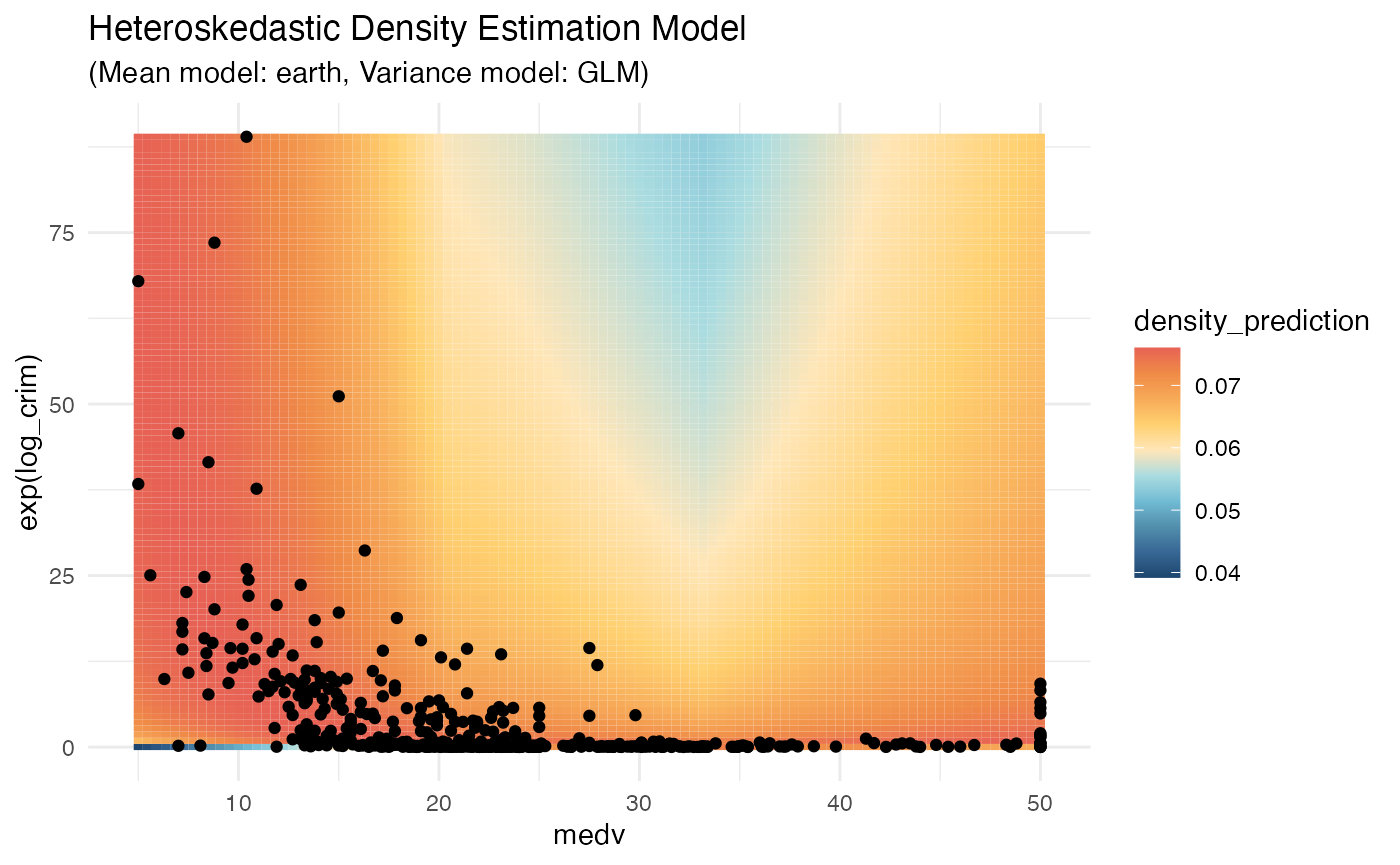
The above example is in 2D (e.g., one predictor and one outcome
variable), but in practical settings we may be estimating the density
for one variable conditional on many other variables. The syntax easily
extends as follows, recalling that reg_formula was
instantiated above as ~, crim, ..
lnr_earth_glm_heteroskedastic_density <- function(data, formula, ...) {
  lnr_heteroskedastic_density(data, formula, mean_lnr = lnr_earth,
                            var_lnr = lnr_mean,
                            density_args = list(bw = 3),
                            ...)
}

lnr_earth_glm_heteroskedastic_predict <-
  lnr_earth_glm_heteroskedastic_density(Boston, reg_formula)

lnr_earth_glm_heteroskedastic_predict(Boston[1,])
#> [1] 0.1280906

f_earth_mean <- function(ys) {
  x <- Boston[1,]
  sapply(ys, function(y) {
    x[['crim']] <- y
    lnr_earth_glm_heteroskedastic_predict(x)
  })
}

integrate(f_earth, min(Boston$crim) - sd(Boston$crim), max(Boston$crim) + sd(Boston$crim))
#> 0.6147477 with absolute error < 5.8e-05
We’ve omitted visualizing what the predictions look like for this model. In general, while it can be useful to spot check whether or not integration is working correctly, or if certain heuristics hold, it can be hard to reason about how a 2D slice of a higher dimensional conditional density model should appear.
For example, some intuition that begins to fail in higher dimensional conditional density models is that the density should be higher where the data points are clustered: if one conditions on a set of all but 2 parameter values and visualizes a grid like in the above example for the remaining predictor and outcome variables, the set of variables conditioned on may be more consistent with higher density in a region outside the bulk of the data distribution if the conditioning set is more consistent with outliers.
In general, this is why for higher dimensional models, we prefer to rely on checks like “does the density integrate to 1?” after conditioning on a full set of predictors and integrating over the possible values of the outcome.
2D Density Estimation
Perhaps visualizing density estimation in 2-to-3 dimensions will help people understand what’s going on.
Suppose our regression problem is to regress flipper length on bill depth from the palmer penguins dataset. We’ll fit some conditional density models and visualize their predictions.
library(palmerpenguins)
library(MetBrewer)

data <- penguins[,c('flipper_length_mm', 'bill_depth_mm')]
data <- data[complete.cases(data),]

# conditional normal example:

learned_conditional_normal <- lnr_lm_density(data, flipper_length_mm ~ bill_depth_mm)

prediction_grid <- expand.grid(
  flipper_length_mm = seq(172, 231, length.out = 100),
  bill_depth_mm = seq(13.1, 21.5, length.out = 100))

prediction_grid$density_prediction <- learned_conditional_normal(prediction_grid)

ggplot(data, aes(x = bill_depth_mm, y = flipper_length_mm)) +
  geom_tile(
    data = prediction_grid,
    mapping = aes(fill = density_prediction)) +
  geom_point() +
  theme_minimal() +
  MetBrewer::scale_fill_met_c('Hiroshige', direction = -1) +
  ggtitle("Conditionally Normal Density Model")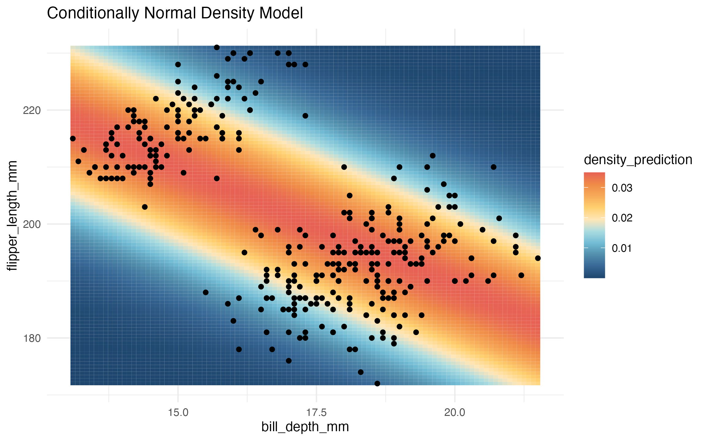
# earth and stats::density

learned_earth_homoskedastic_density <-
  lnr_earth_homoskedastic_density(data, flipper_length_mm ~ bill_depth_mm)

prediction_grid$density_prediction <- learned_earth_homoskedastic_density(prediction_grid)

ggplot(data, aes(x = bill_depth_mm, y = flipper_length_mm)) +
  geom_tile(
    data = prediction_grid,
    mapping = aes(fill = density_prediction)) +
  geom_point() +
  theme_minimal() +
  MetBrewer::scale_fill_met_c('Hiroshige', direction = -1) +
  ggtitle("Using earth::earth for conditional mean and stats::density for error")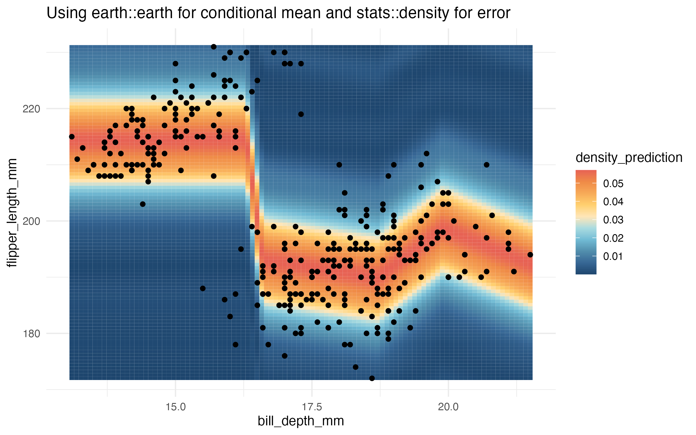
# randomForest and stats::density

learned_rf_homoskedastic_density <-
  lnr_rf_homoskedastic_density(data, flipper_length_mm ~ bill_depth_mm)

prediction_grid$density_prediction <- learned_rf_homoskedastic_density(prediction_grid)

ggplot(data, aes(x = bill_depth_mm, y = flipper_length_mm)) +
  geom_tile(
    data = prediction_grid,
    mapping = aes(fill = density_prediction)) +
  geom_point() +
  theme_minimal() +
  MetBrewer::scale_fill_met_c('Hiroshige', direction = -1) +
  ggtitle("Using randomForest::randomForest for conditional mean and stats::density for error")
# ranger and stats::density

learned_ranger_homoskedastic_density <-
  lnr_ranger_homoskedastic_density(data, flipper_length_mm ~ bill_depth_mm)

prediction_grid$density_prediction <- learned_ranger_homoskedastic_density(prediction_grid)

ggplot(data, aes(x = bill_depth_mm, y = flipper_length_mm)) +
  geom_tile(
    data = prediction_grid,
    mapping = aes(fill = density_prediction)) +
  geom_point() +
  theme_minimal() +
  MetBrewer::scale_fill_met_c('Hiroshige', direction = -1) +
  ggtitle("Using ranger::ranger for conditional mean and stats::density for error")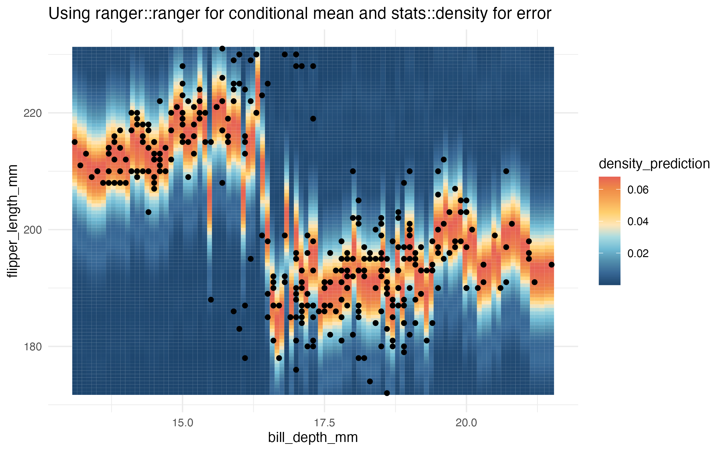
# glm and stats::density

learned_glm_homoskedastic_density <-
  lnr_homoskedastic_density(data, flipper_length_mm ~ bill_depth_mm, mean_lnr = lnr_glm)

prediction_grid$density_prediction <- learned_glm_homoskedastic_density(prediction_grid)

ggplot(data, aes(x = bill_depth_mm, y = flipper_length_mm)) +
  geom_tile(
    data = prediction_grid,
    mapping = aes(fill = density_prediction)) +
  geom_point() +
  theme_minimal() +
  MetBrewer::scale_fill_met_c('Hiroshige', direction = -1) +
  ggtitle("Using stats::glm for conditional mean and stats::density for error")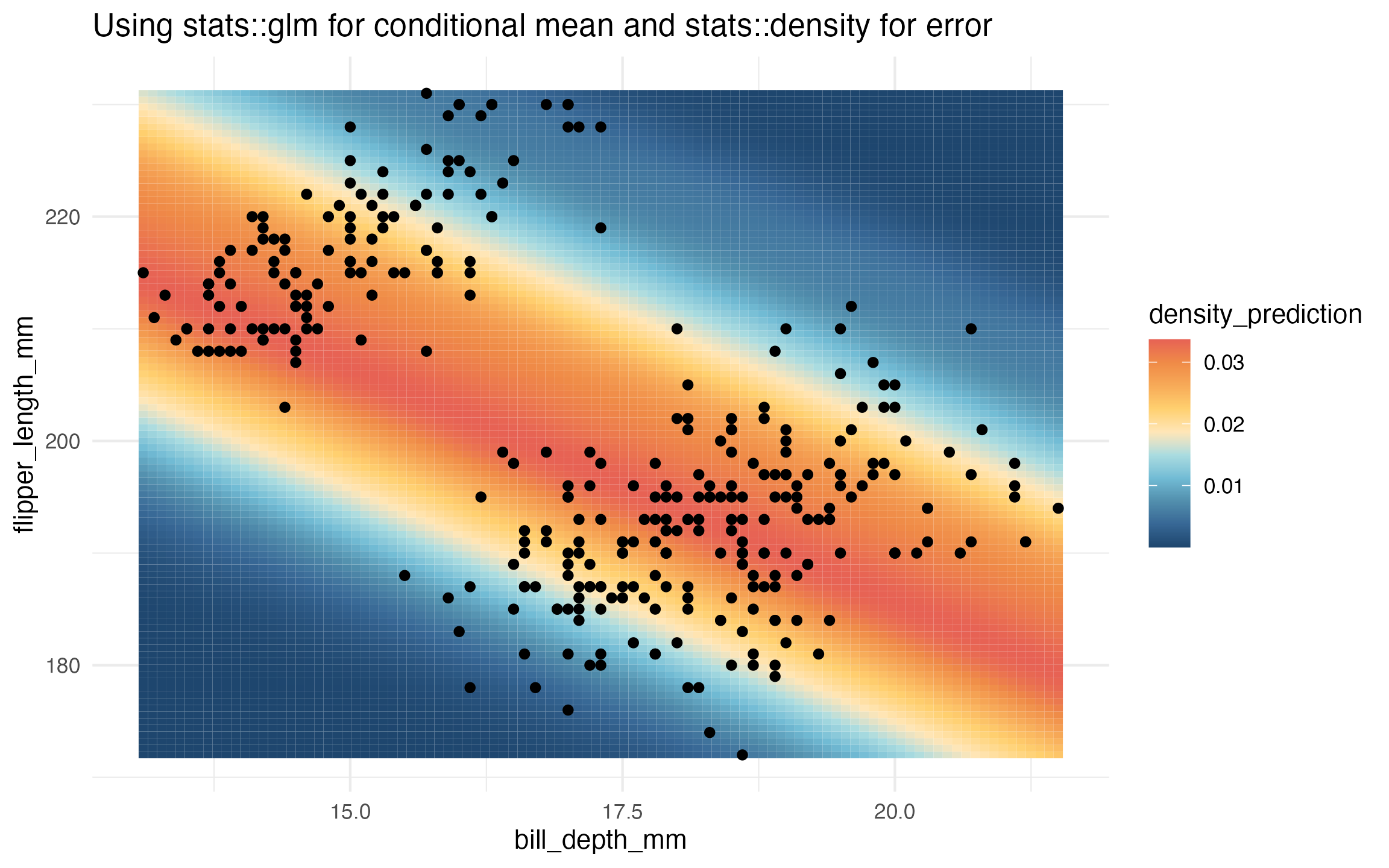
#  heteroskedastic method

learned_earth_heteroskedastic_density <-
  lnr_heteroskedastic_density(data,
                              flipper_length_mm ~ bill_depth_mm,
                              mean_lnr = lnr_earth,
                              var_lnr = lnr_glm)

prediction_grid$density_prediction <- learned_earth_heteroskedastic_density(prediction_grid)

ggplot(data, aes(x = bill_depth_mm, y = flipper_length_mm)) +
  geom_tile(
    data = prediction_grid,
    mapping = aes(fill = density_prediction)) +
  geom_point() +
  theme_minimal() +
  MetBrewer::scale_fill_met_c('Hiroshige', direction = -1) +
  ggtitle("Using earth::earth for conditional mean, stats::density for error distribution, \nand a stats::glm for predicting heteroskedasticity")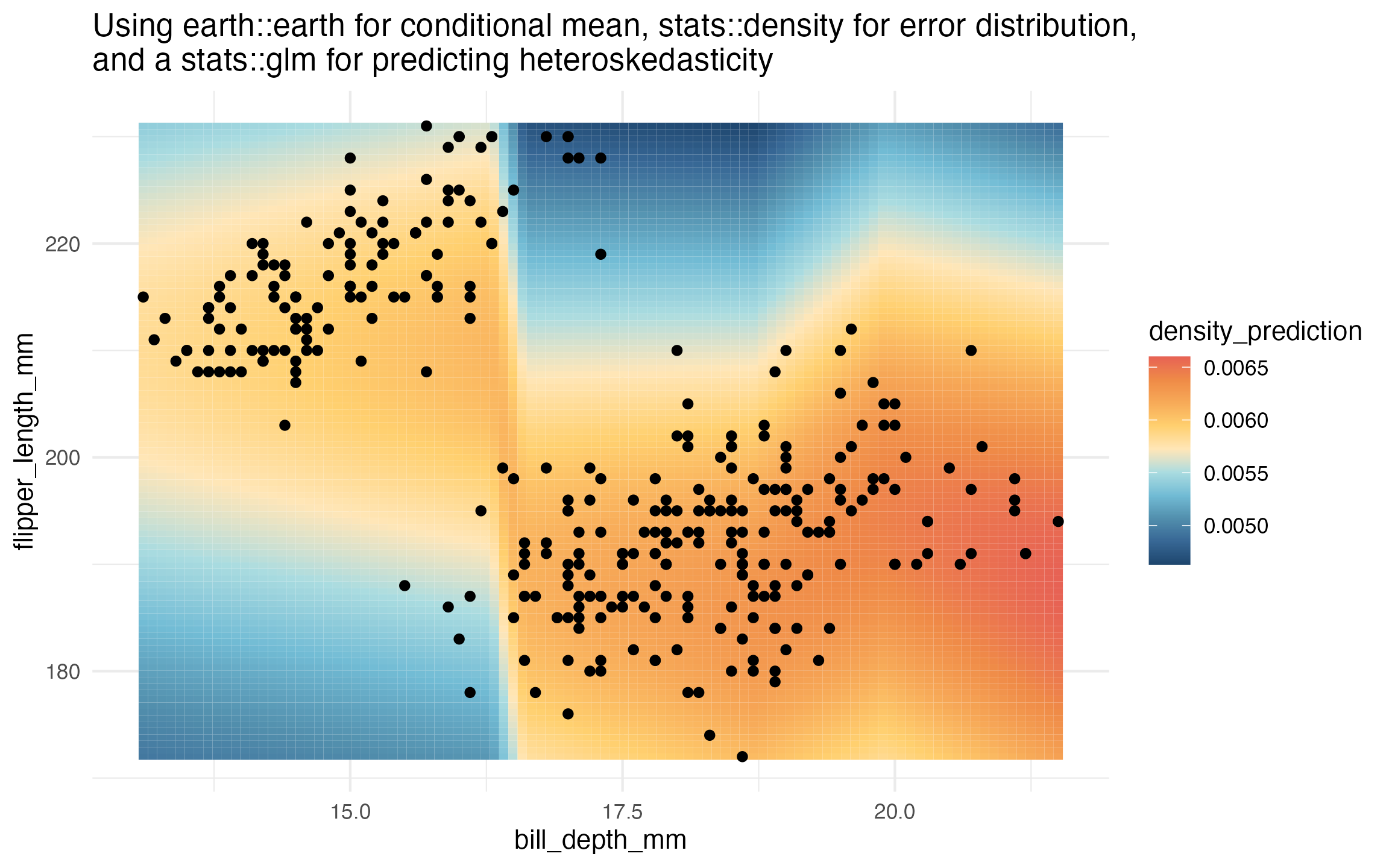
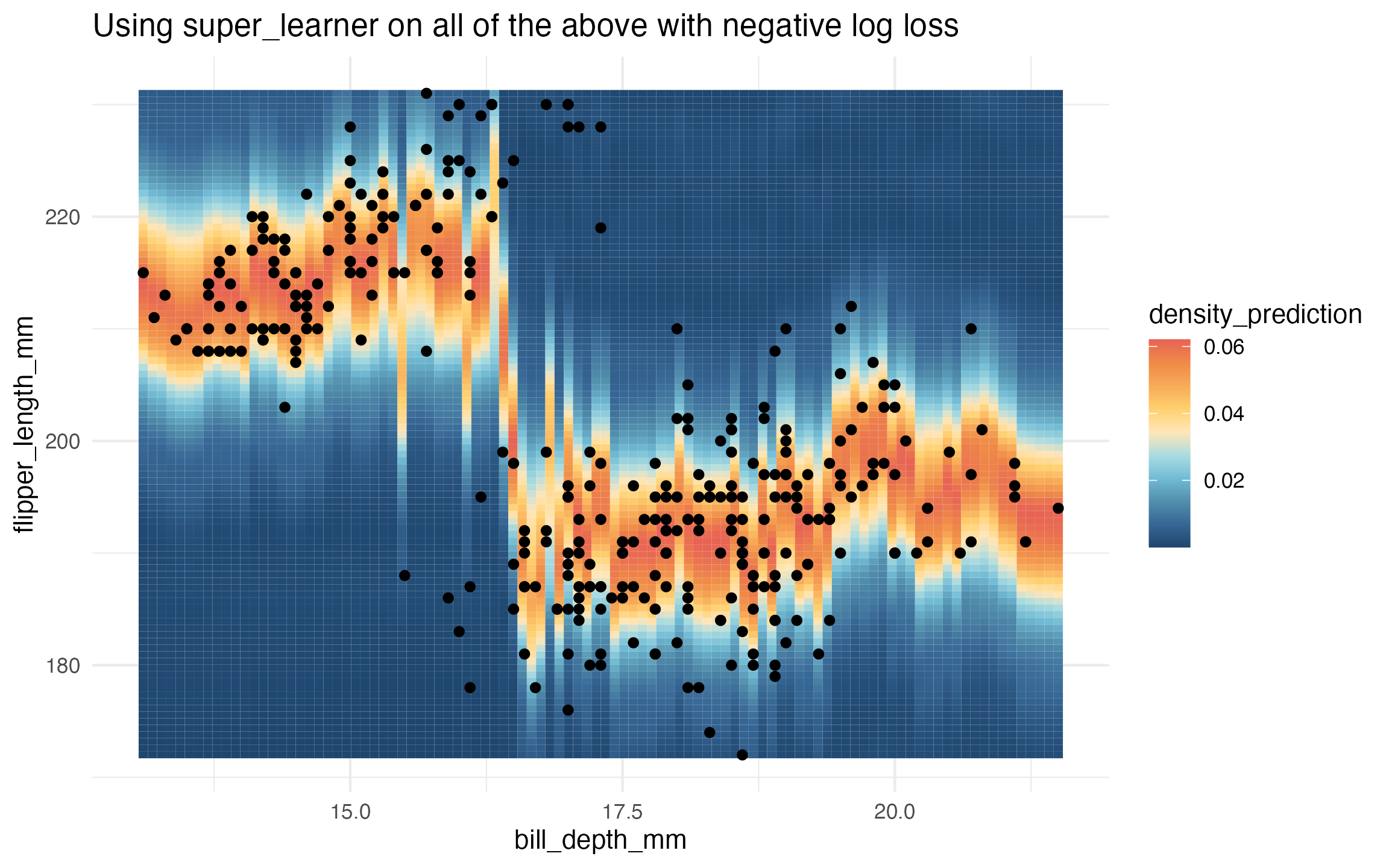
# super learner

learned_sl_density <-
  super_learner(data,
    flipper_length_mm ~ bill_depth_mm,
    learners = list(
      lm = lnr_lm_density,
      earth = lnr_earth_homoskedastic_density,
      rf = lnr_rf_homoskedastic_density,
      ranger = lnr_ranger_homoskedastic_density,
      heteroskedastic = lnr_heteroskedastic_density
      ),
    extra_learner_args = list(
      heteroskedastic = list(mean_lnr = lnr_earth, var_lnr = lnr_glm)
      ),
    determine_super_learner_weights = determine_weights_using_neg_log_loss)
#> Warning in validate_learner_types(learners, outcome_type): Learners 1, 2, 3, 4, 5 with names [lm, earth, rf, ranger, heteroskedastic] do not have attr(., 'sl_lnr_type') == 'continuous'.
#> See the Creating Learners article on the {nadir} website.
#>

prediction_grid$density_prediction <- learned_sl_density(prediction_grid)

ggplot(data, aes(x = bill_depth_mm, y = flipper_length_mm)) +
  geom_tile(
    data = prediction_grid,
    mapping = aes(fill = density_prediction)) +
  geom_point() +
  theme_minimal() +
  MetBrewer::scale_fill_met_c('Hiroshige', direction = -1) +
  ggtitle("Using super_learner on all of the above with negative log loss")