Visualizing Performance

nadir model objects come with plot() methods, so visualizing how your candidate learners and the super learner ensemble performed takes one line of code. This article tours the available plot types and explains which comparison is the fair comparison to make.

library(nadir)

Throughout we’ll use the Boston housing data and a moderately diverse library of learners:

data("Boston", package = "MASS")

learners <- list(
  lm = lnr_lm,
  rf = lnr_rf,
  ranger = lnr_ranger,
  xgboost = lnr_xgboost,
  glmnet = lnr_glmnet,
  earth = lnr_earth
)

sl_model <- super_learner(
  data = Boston,
  formulas = medv ~ .,
  learners = learners
)
#> Warning: package 'future' was built under R version 4.5.2

Comparing the candidate learners

compare_learners() reports each candidate’s cross-validated held-out loss as a table:

compare_learners(sl_model)
#> Inferring the loss metric for learner comparison based on the outcome type:
#> outcome_type=continuous -> using mean squared error
#> # A tibble: 1 × 6
#>      lm    rf ranger xgboost glmnet earth
#>   <dbl> <dbl>  <dbl>   <dbl>  <dbl> <dbl>
#> 1  23.9  10.6   11.3    11.0   25.5  14.6

The default plot() method shows the same information visually, along with how variable each learner’s performance was across the cross-validation folds:

plot(sl_model)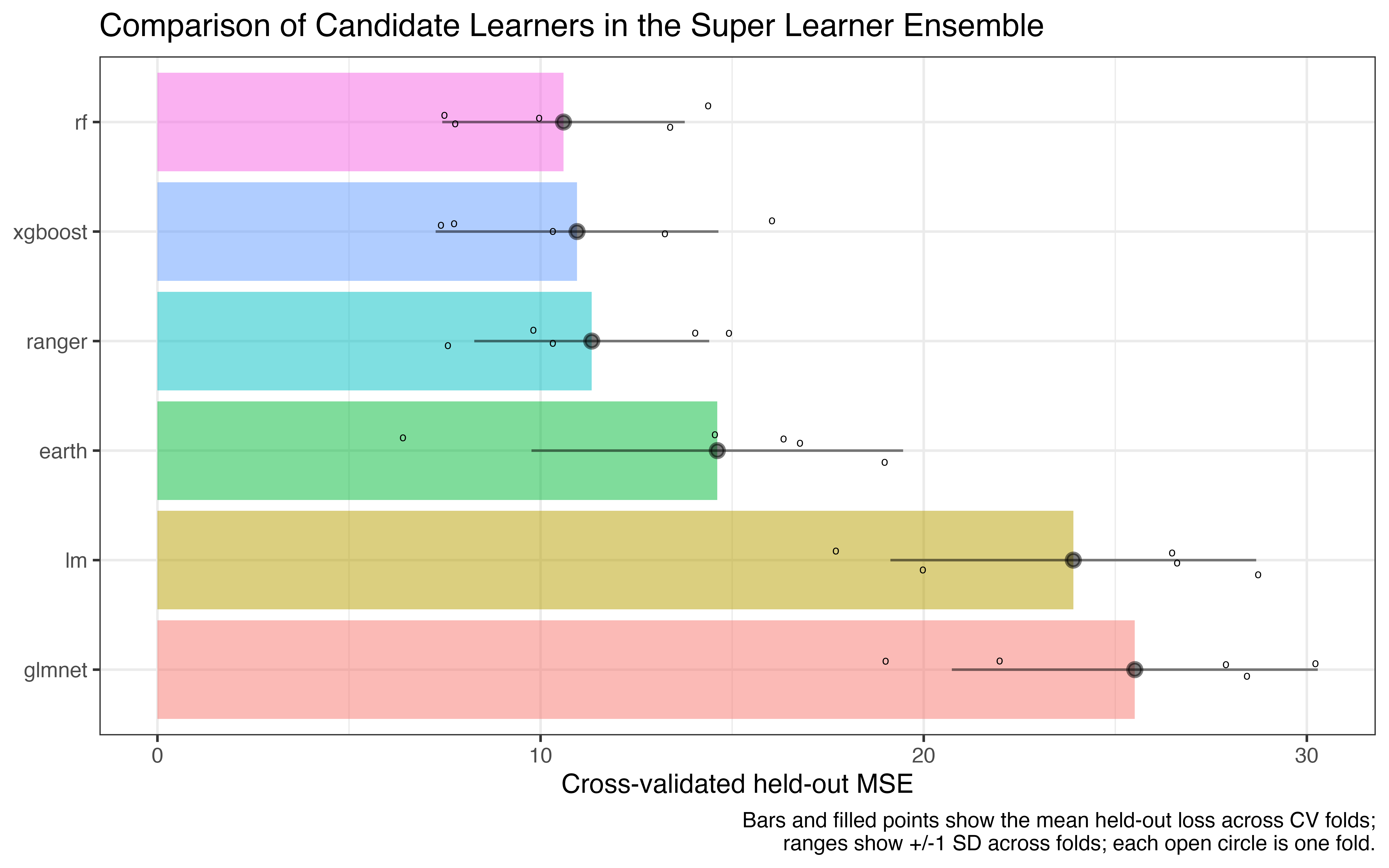

For each candidate learner, the bar and filled point show the mean held-out loss across the cross-validation folds, each circle mark shows one fold’s held-out loss, and the range shows plus or minus 1 standard deviation across folds. Learners are ordered best (lowest mean loss) at the top.

So where is super learner in this plot?

Without additional work, we can’t fairly judge super learner yet because we don’t have the super learner’s held-out loss value.

A super_learner() fit chooses its ensemble weights using the candidates’ holdout predictions, so scoring the ensemble on those same holdouts would be optimistically biased. The ensemble gets to see the data that it would be evaluated on. plot(sl_model) therefore compares only the candidates, which were each scored honestly on held out data.

To score the ensemble itself fairly, we need another layer of cross-validation. That’s the purpose of cv_super_learner().

Honestly evaluating the super learner

cv_results <- cv_super_learner(
  data = Boston,
  formulas = medv ~ .,
  learners = learners
)

plot(cv_results)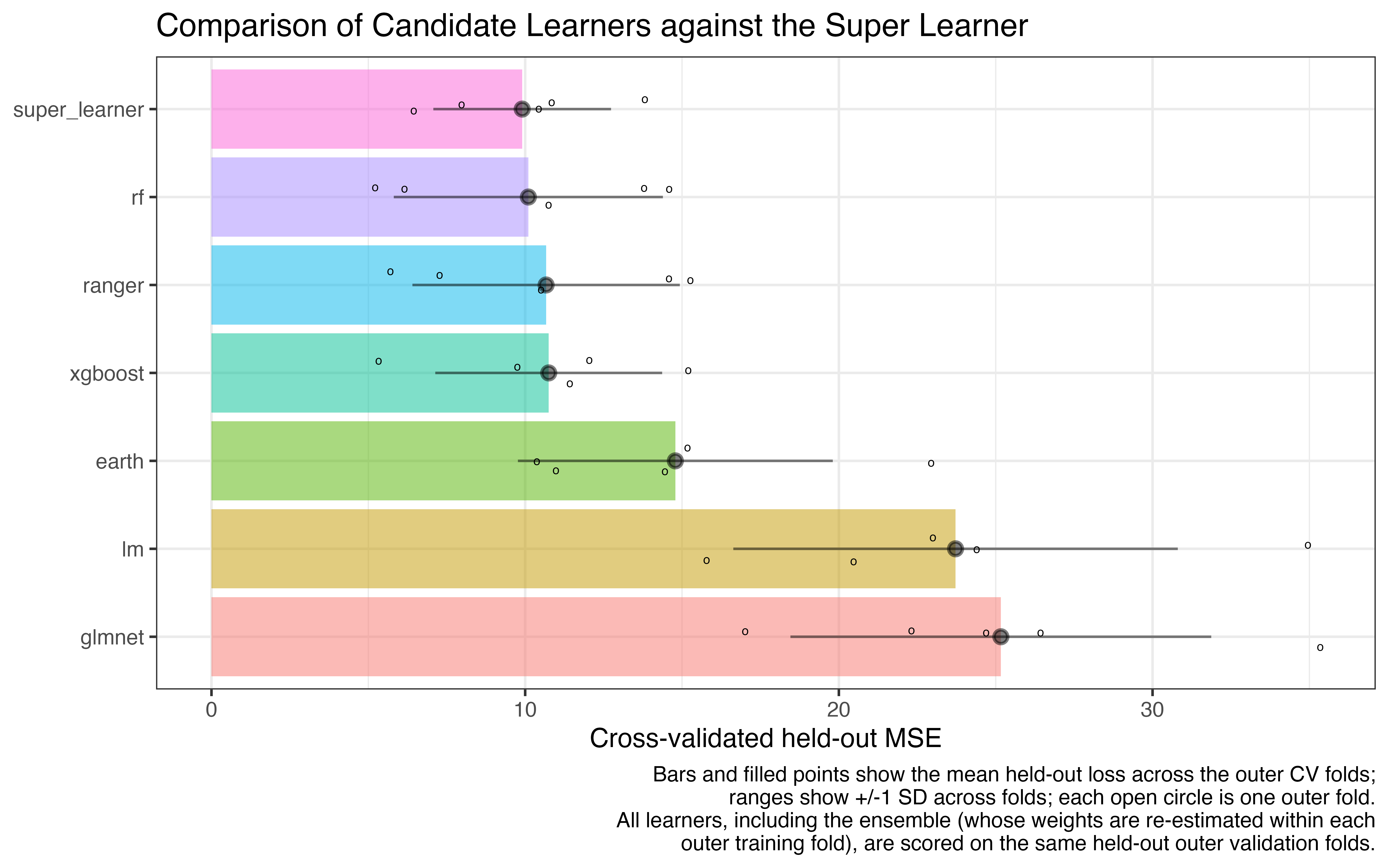

Now the super_learner row appears alongside the candidates, and the comparison is a level playing field: within each outer fold, the candidate fits and the ensemble weights were all estimated entirely without the validation data they’re evaluated on, and every learner was trained on the same outer training data.

Ensemble weight stability

How consistently does the super learner weight its candidates when the training data changes? type = "weights" shows the ensemble weights estimated within each outer fold:

plot(cv_results, type = "weights")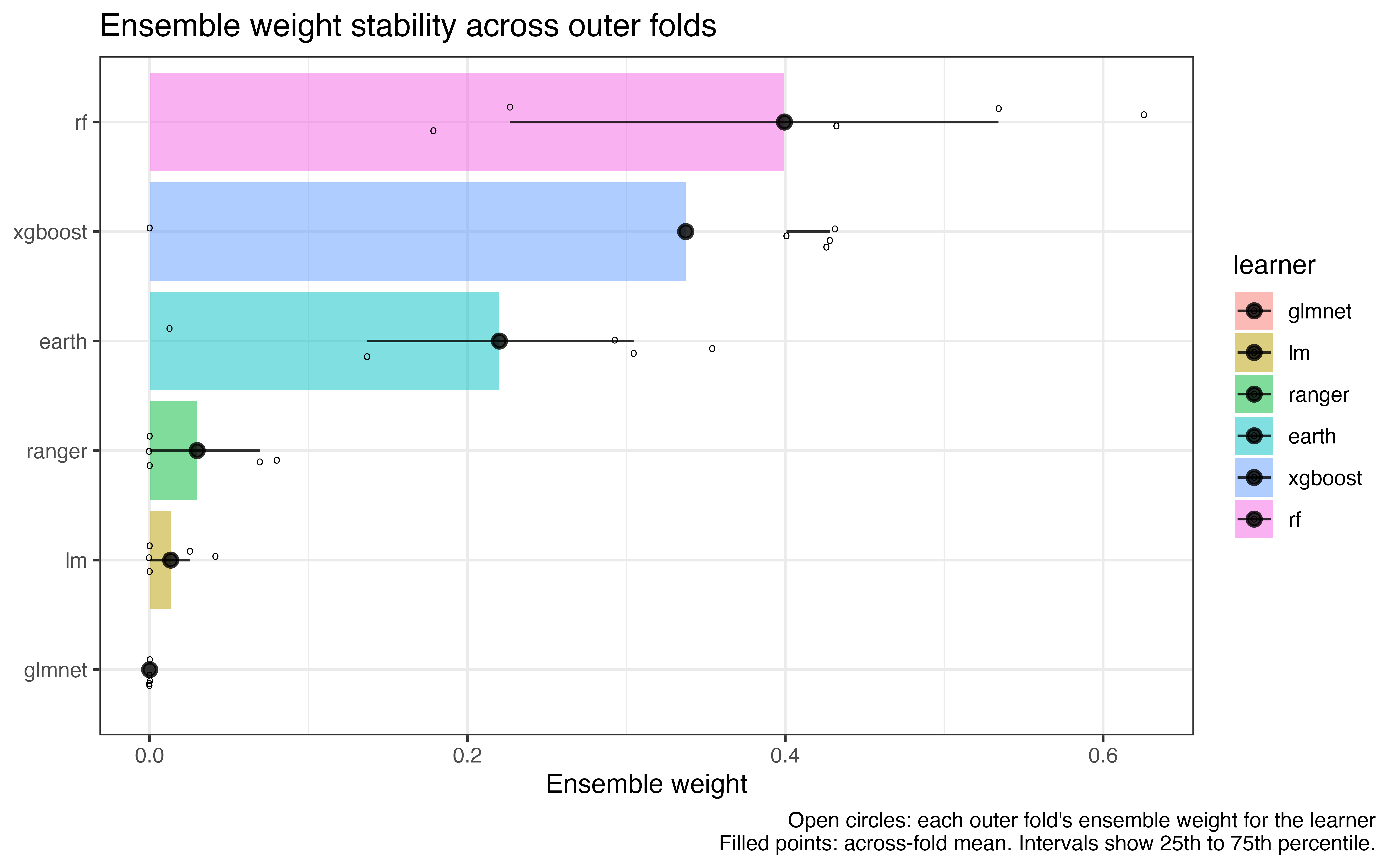

Tight clusters indicate an ensemble that is stable under resampling. If a learner’s weights vary wildly from fold to fold, that’s a sign the data don’t strongly distinguish it from its competitors (or that it’s unstable); missing points would indicate folds where a learner errored and was dropped.

Predictions vs. observed outcomes

Finally, type = "fitted" plots out-of-fold ensemble predictions against the observed outcomes, with the identity line for reference:

plot(cv_results, type = "fitted")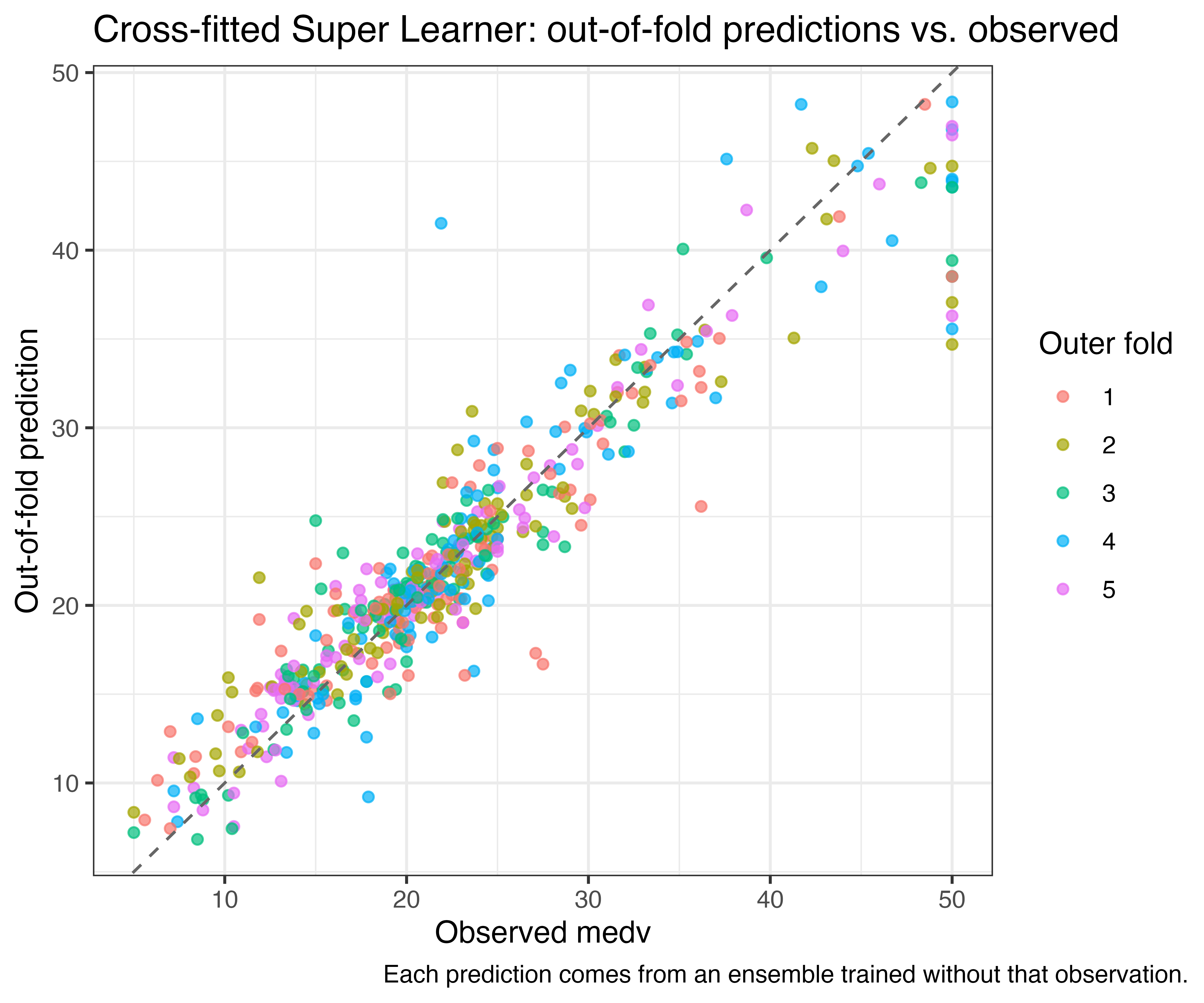

Every prediction here comes from an ensemble trained entirely without that observation, so systematic deviations from the identity (45-degree) line would reflect shortcomings of the overall super learned model fit. The same view is available for a plain super_learner() fit via plot(sl_model, type = "fitted"), using its cross-validated holdout predictions.

Customizing the plots

Each plot() method returns a ggplot object, so the usual ggplot2 grammar applies if you want to restyle them:

plot(cv_results) +
  ggplot2::scale_fill_brewer(palette = "Set2") +
  ggplot2::theme_minimal()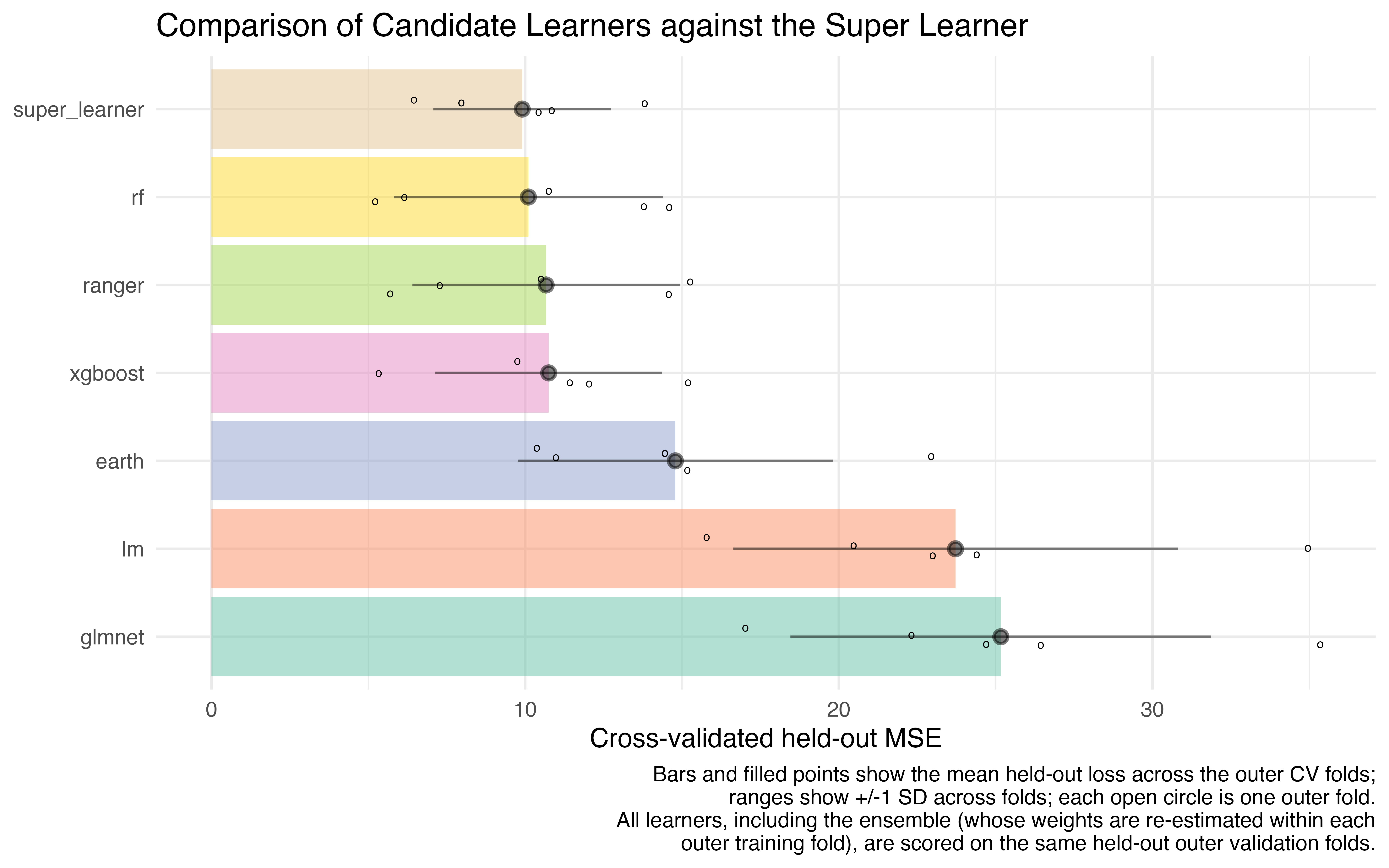

If you need something the plot methods don’t offer, the raw materials are all retained on the fitted objects: per-fold holdout predictions live in sl_model$holdout_predictions, and the per-fold super_learner() fits from the outer cross-validation live in cv_results$crossfit.