Timing Learners via the Warning System

nadir::super_learner() never lets learner warnings hit your console: every warning signaled during training or prediction is muffled, captured, and returned to you in $warnings_from_training_cv_stage1, $warnings_from_predicting_cv_stage2, and $warnings_from_training_on_entire_data, each a list of warning condition objects named by the learner that signaled them.

A fun consequence: since warnings are captured as full condition objects (not just messages), the warning system doubles as a structured side-channel out of the training stage. Anything a learner wants to report about its own fitting process — without disturbing its return value, which must remain a prediction function — can be smuggled out as a classed warning condition carrying extra fields.

In this vignette we use that side-channel to answer a practical question: which of my candidate learners are the slowest to fit? We’ll write a learner-modifier, add_learner_timing_warnings(), in the same spirit as nadir::add_screener(): it takes a learner and returns a new learner that behaves identically, except that it times its training step and signals a formatted warning carrying the timing results.

library(nadir)
library(ggplot2)
#> Warning: package 'ggplot2' was built under R version 4.5.2

Building `add_learner_timing_warnings()`

First, a small constructor for our custom warning condition. Giving the condition its own class, learner_timing_warning, is what lets us later distinguish deliberate timing warnings from any organic warnings the learners happen to throw (rank-deficiency complaints, convergence grumbles, and so on). Alongside the human-readable message, we stash the raw elapsed seconds and the learner’s name as structured fields, so no message-parsing is needed downstream.

learner_timing_warning <- function(learner_name, timing) {
  structure(
    class = c("learner_timing_warning", "warning", "condition"),
    list(
      message = sprintf(
        "[learner timing] %s: trained in %.3f seconds (elapsed) on %s",
        learner_name,
        timing[["elapsed"]],
        format(Sys.time(), "%H:%M:%OS2")
      ),
      call = sys.call(-1),
      learner_name = learner_name,
      elapsed = unname(timing[["elapsed"]])
    )
  )
}

Now the modifier itself. Like all nadir learners, the wrapped version is a function factory taking (data, formula, ...) and returning a prediction function; the only change is a system.time() around the training call and a warning() signaling our classed condition afterwards. We copy over the sl_lnr_name and sl_lnr_type attributes so that automatic learner naming and outcome-type checking keep working exactly as they would for the unwrapped learner.

add_learner_timing_warnings <- function(learner) {
  learner_name <- attr(learner, "sl_lnr_name")
  if (is.null(learner_name)) {
    learner_name <- "unnamed_lnr"
  }

  timed_learner <- function(data, formula, ...) {
    timing <- system.time({
      trained_predictor <- learner(data = data, formula = formula, ...)
    })
    warning(learner_timing_warning(learner_name, timing))
    return(trained_predictor)
  }

  attr(timed_learner, "sl_lnr_name") <- learner_name
  attr(timed_learner, "sl_lnr_type") <- attr(learner, "sl_lnr_type")
  return(timed_learner)
}

Note that because super_learner() muffles the warnings it captures, wrapping learners this way adds no console noise at all — even under parallel future plans, where the capture happens inside the workers before results are collected.

Fitting a super learner on the `penguins` data

We’ll use the complete cases of the palmerpenguins data and a library of six learners of rather different computational temperaments, from the essentially free lnr_mean up through random forests and gradient boosting.

penguins <- palmerpenguins::penguins
penguins <- penguins[complete.cases(penguins), ]

flipper_length_formula <-
  flipper_length_mm ~ species + island + bill_length_mm +
  bill_depth_mm + body_mass_g + sex

timed_learners <- lapply(
  list(
    lnr_mean, lnr_lm, lnr_rf, lnr_earth, lnr_cvglmnet, lnr_xgboost,
    lnr_svm, lnr_bart, lnr_lightgbm, lnr_ranger,
    lnr_earth
  ),
  add_learner_timing_warnings
)

set.seed(2026)
sl_model <- super_learner(
  data = penguins,
  formula = flipper_length_formula,
  learners = timed_learners
)
#> Warning: package 'future' was built under R version 4.5.2

Nothing was printed — but the timing warnings were captured. With the default n_folds = 5, each learner signals five warnings during the cross-validation training stage (one per training fold), plus one more when it is refit on the entire dataset:

length(sl_model$warnings_from_training_cv_stage1)
#> [1] 55
length(sl_model$warnings_from_training_on_entire_data)
#> [1] 11

# the warnings are named by learner, and the messages are human-readable:
conditionMessage(sl_model$warnings_from_training_cv_stage1[[1]])
#> [1] "[learner timing] mean: trained in 0.000 seconds (elapsed) on 12:29:00.54"

Extracting the timing warnings

Now we harvest our deliberate warnings back out. We filter each warning field for conditions inheriting from learner_timing_warning — leaving any organic learner warnings untouched — and assemble the structured $elapsed fields into a tidy data frame.

extract_learner_timings <- function(sl_model) {
  warning_fields <- c(
    cv_training = "warnings_from_training_cv_stage1",
    full_data_fit = "warnings_from_training_on_entire_data"
  )

  do.call(rbind, lapply(names(warning_fields), function(stage) {
    warnings_list <- sl_model[[warning_fields[[stage]]]]
    timing_warnings <- Filter(
      function(w) inherits(w, "learner_timing_warning"),
      warnings_list
    )
    if (length(timing_warnings) == 0) {
      return(NULL)
    }
    data.frame(
      learner = vapply(timing_warnings, `[[`, character(1), "learner_name"),
      stage = stage,
      elapsed = vapply(timing_warnings, `[[`, numeric(1), "elapsed")
    )
  }))
}

learner_timings <- extract_learner_timings(sl_model)
head(learner_timings)
#>   learner       stage elapsed
#> 1    mean cv_training   0.000
#> 2    mean cv_training   0.000
#> 3    mean cv_training   0.000
#> 4    mean cv_training   0.000
#> 5    mean cv_training   0.000
#> 6      lm cv_training   0.002

Visualizing which learners are fastest to fit

Averaging the per-fold training times gives us a bar chart of mean time-to-fit per learner, with the individual fold timings overlaid as points so the fold-to-fold variability is visible too.

cv_timings <- learner_timings[learner_timings$stage == "cv_training", ]

mean_timings <- aggregate(elapsed ~ learner, data = cv_timings, FUN = mean)
mean_timings$learner <- reorder(mean_timings$learner, mean_timings$elapsed)
cv_timings$learner <- factor(cv_timings$learner, levels = levels(mean_timings$learner))

ggplot(mean_timings, aes(x = elapsed, y = learner, fill = learner)) +
  geom_col(alpha = .8) +
  geom_point(data = cv_timings, shape = 21, fill = "white", alpha = .75) +
  # scale_fill_brewer(palette = 'Set2', guide = 'none') +
  scale_fill_brewer(palette = "BrBG", guide = "none") +
  theme_bw() +
  labs(
    x = "mean elapsed training time per fold (seconds)",
    y = NULL,
    title = "Time-to-fit for each candidate learner",
    subtitle = "Bars show the mean across the 5 CV training folds; points show individual folds",
    caption = "Task: flipper_length_mm ~ . on the penguins complete cases, 333 rows.
Timings harvested from deliberately-signaled learner_timing_warning conditions
captured by nadir::super_learner()'s warning system."
  ) +
  theme(plot.caption.position = "plot")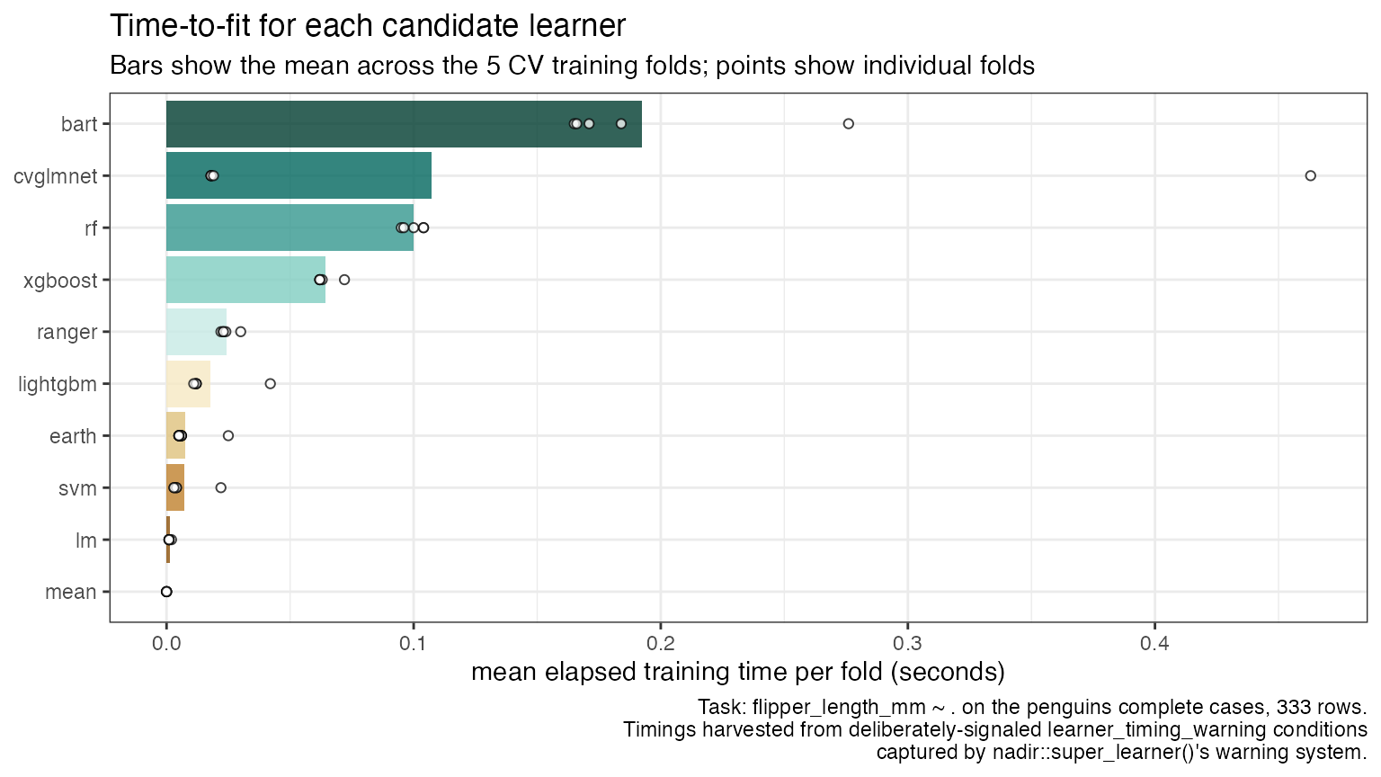

Unsurprisingly, lnr_mean and lnr_lm are effectively free, while the tree-ensemble learners dominate the fitting budget. Since timing warnings are signaled once per training call, this approach extends without modification to cv_super_learner() and crossfit_super_learner(), whose outputs aggregate the same captured-warning fields across their outer folds.

Two closing remarks on the pattern itself. First, a warning is not an error: a timing-wrapped learner keeps its weight-eligibility, its predictions, and its place in the ensemble entirely unchanged — we can confirm the wrapped learners were named and weighted as usual:

round(sl_model$learner_weights, 3)
#>     mean       lm       rf  earth_1 cvglmnet  xgboost      svm     bart 
#>    0.000    0.311    0.366    0.000    0.000    0.000    0.277    0.046 
#> lightgbm   ranger  earth_2 
#>    0.000    0.000    0.000

Second, nothing about this trick is specific to timing. Any per-fit diagnostic — memory use, number of boosting rounds actually run, screening decisions — can ride the same classed-condition side-channel out of the training stage and back to you through super_learner()’s captured warnings.

Building add_learner_timing_warnings()

Fitting a super learner on the penguins data

Extracting the timing warnings

Visualizing which learners are fastest to fit

Building `add_learner_timing_warnings()`

Fitting a super learner on the `penguins` data